 MR执行流
MR执行流
Introduction
MapReduce is a concept proposed in a paper published by Google in 2004 (Google internally wrote the first version in 2003). Although fifteen years have passed, looking back at the background, principles, and implementation of this ancestor-level concept of the big data era still yields many intuitive insights into distributed systems — as the saying goes, one can learn new things by reviewing the old.
In Google’s context, MapReduce is both a programming model and a distributed system implementation supporting that model. Its proposal allowed developers without a distributed systems background to easily harness large-scale clusters to process massive amounts of data with high throughput. Its problem-solving approach is well worth learning from: identify the pain points of the requirements (e.g., how to maintain, update, and rank massive indexes), perform high-level abstraction of key processing workflows (shard via Map, reduce on demand), and carry out efficient system implementation (tailored to fit). Among these, finding a suitable computational abstraction is the hardest part, requiring both an intuitive understanding of requirements and extremely high computer science literacy. Of course, and perhaps closer to reality, this abstraction is the tip of the iceberg above the water, evolved through constant trial and error based on requirements.
Author: QtMuniao https://www.qtmuniao.com, please credit when reposting
Motivation
At that time, as the largest gateway to the Internet, Google maintained the entire web index of the world and was the first to hit the ceiling of data volume. That is, even for very simple business logic — such as generating inverted indexes from crawl data, organizing the graph-like web page collection in different ways, calculating the number of crawled web pages per host, or high-frequency query terms for a given date — the scale of global Internet data made it exceptionally complex.
These complexities included: input data scattered across a great many hosts, computations too resource-intensive for a single machine to complete, and output data needing to be reorganized across hosts. As a result, it was necessary to repeatedly construct dedicated systems for each requirement and spend a lot of code on distributing data and code, scheduling and parallelizing tasks, handling machine failures, and dealing with communication failures.
Abstraction
The abstraction of map and reduce was inspired by the functional programming language Lisp. Why were these two concepts chosen? It stems from the Googlers’ high-level refinement of their business: first, the input can be split into logical records; then for each record, perform a mapping (map) operation to generate intermediate results composed of key-value pairs (why split into keys and values? To pave the way for the final step, allowing users to organize and reduce the intermediate results in any specified way — by key); finally, perform a reduction (reduce, including sorting, statistics, extracting extrema, etc.) on the subset of intermediate results with the same key.
Another characteristic of the functional model is the constraint on the implementation of the map operation, which stipulates that users should provide a side-effect-free map operation (related concepts include pure functions, determinism, idempotency, etc.; of course, their concepts are not identical, which will be discussed in detail later). Such restrictions have two benefits: it enables massive parallel execution, and it allows masking machine failures by retrying elsewhere.
Specifically, for implementation, both map and reduce are user-defined functions. The map function accepts a Record; however, for flexibility, it is generally also organized as a key-value pair, and then produces List[key, value]. The reduce function accepts a key and all intermediate results List[value] corresponding to that key. That is:
1 | map (k1,v1) -→ list(k2,v2) |
Take the Word Count example program (counting words in a bunch of documents), proposed by Google’s paper and later becoming the hello world of the big data processing world. The implementations of map and reduce look like this:
1 | map(String key, String value): |
Here are two interesting points:
- Intermediate variables need network transmission, which inevitably involves serialization. The initial version of MapReduce chose to leave all interpretation to the runtime user code — it simply passed strings. That is, users were required to convert any output intermediate result objects into strings in map, and then after receiving Iterator[string] in the reduce function, parse it into the desired format themselves. Of course, in later imitation frameworks such as Hadoop, the serialization and deserialization parts were extracted and could be customized by users to meet functional or performance requirements. I didn’t verify this, but presumably Google later optimized this as well. This is a very natural system evolution approach: the initial design should be as simple and crude as possible to quickly implement a usable prototype; after accumulating usage experience, certain inconvenient modules can be extended.
- The value collection received by reduce is organized as an Iterator. Those who have used Python should be familiar with iterators. It is a very simple interface, including next and stop semantics. Combined with a for loop, it forms a very powerful abstraction. Whether the underlying layer is a List in memory, file contents, or a network IO stream, as long as the runtime knows how to get the next record and when to stop, it can be utilized by a for loop for sequential processing. One advantage of the iterator abstraction is that it does not need to load all content to be iterated into memory at once; it can perform incremental lazy loading of data. The MapReduce framework’s implementation here also leverages this characteristic.
Implementation Overview
Once the abstraction is defined, the implementation can naturally vary — this is the meaning of separation of interface and implementation. The former abstraction is an idea that Google has already provided; the latter implementation can be completely tailored according to one’s own production environment. In its paper, Google presented a classic internal version, and Hadoop also provides a general-purpose version; of course, we can also implement a custom-fitted version according to our own business requirements and scenario constraints.
The system environment that Google faced when publishing the paper for implementing MapReduce looked like this:
- Single machine with dual-core x86 architecture, 2~4GB memory, Linux system
- Commodity network hardware, 100 Mbps or Gigabit Ethernet
- Clusters containing hundreds or thousands of machines, so machine failures were the norm
- Cheap IDE interface hard drives, but they had GFS to provide fault tolerance
- Multi-tenant support, so job-level abstraction and resource constraints were needed
Workflow Overview
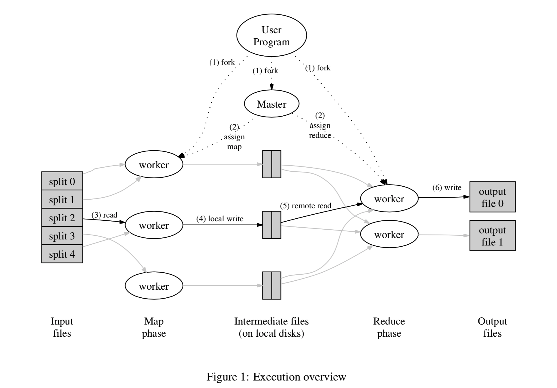
After the user specifies the split size, the input is divided into M pieces and distributed across different machines (due to the presence of GFS, the input block may already be on that machine). On each machine, the user-defined map runs in parallel. The intermediate results output by map are also specified by the user to be divided into R pieces by key value range. For each intermediate result, its destination is determined by node label = hash(key) mod R. Below is a workflow overview diagram:
MR执行流
- First, the input is divided into M pieces, usually 16~64M each; the user controls this granularity as needed. Then these splits are distributed across different machines (if coordinated with a distributed file system like GFS, they may already be distributed), and the user’s code is forked on each machine. User code distribution is an interesting topic; different languages may have different implementations. For example, Google’s C++ might transmit dynamic link libraries; for Hadoop’s Java, it might transmit jar packages (of course, all dependencies must also be transmitted); for PySpark’s Python, it might use the magical cloudpickle. In short, different languages require different transmission mechanisms, such as dynamic languages versus static languages. In addition, global variables and external dependencies also need to be considered. Although Google glossed over this, the situations faced by different languages may vary greatly.
- The Master’s copy of the program is different — it is responsible for assigning work. It selects idle workers to arrange the M map tasks and R reduce tasks. One consideration here is whether the worker starts a separate process for each user code execution, or inserts it into a system loop to execute.
- The worker executing the map task reads the assigned input split, parses out the key-value stream, and feeds it to the user-defined map function. The temporary results produced by map are first cached in memory. Although the paper does not elaborate, it is foreseeable that how to split and how to parse the key-value stream may differ for different users focusing on the same input, so there must be a need for customized parsing. This part (FileSplit and RecordReader) would likely also be opened up for user customization later as the business grows; in fact, this is exactly what Hadoop did.
- The cached intermediate results are periodically flushed to disk locally on the machine running the Map Task (this is also a locality optimization, but it has consequences — once that machine fails, fault tolerance becomes slightly more troublesome, which will be discussed later), and divided into R blocks according to the user-specified Partition function. Then these location information is sent to the Master node. The Master is responsible for notifying the corresponding Reduce Workers to pull the corresponding data.
- After receiving the location information of these intermediate results, the Reduce Worker pulls the data of the corresponding Partition via RPC. For a certain Reduce Worker, after all data is pulled, it is sorted by key. In this way, all data with the same key is grouped together. The combination of steps 4 and 5 is called shuffle, involving external sorting, multi-machine data transmission, and other extremely time-consuming operations. When the data volume is small, any implementation is fine. But when the data volume reaches a certain scale, this can easily become a performance bottleneck, so there are also some optimization methods. Details on shuffle will be expanded later; for now, we will leave it aside.
- After the intermediate data is sorted, the Reduce Worker scans it, passing each key and its corresponding value set, i.e., <k2, list(v2)>, to the user-customized reduce function, and then appends the generated results to the final output file. For Google, this is generally the parallel-append-capable file system GFS, whose advantage is that multiple processes can write results simultaneously.
- When all reduce tasks are completed, the master wakes up the user process — that is, from the user code’s perspective, the MapReduce task is blocking.
Generally, users do not need to merge the final R partitions, but instead use them directly as input for the next MapReduce task. Spark RDD’s partition conceptually encapsulates this feature, and keeps each MapReduce step’s output in memory without writing to disk, to reduce the latency of continuous MapReduce tasks.
Locality
A commonly used principle in computer science is the locality principle (locality of reference, specifically spatial locality here), which states that when a program executes sequentially and accesses a block of data, it is highly likely to access the block of data adjacent to it (in physical location) next. It is a simple assertion, yet it is the foundation for all caches to function; computer storage thus forms a hierarchical system from slow to fast, from cheap to expensive, and from large to small (hard disk -> memory -> cache -> registers). In a distributed environment, this hierarchy must be covered by at least one more layer — network IO.
In the MapReduce system, we also fully utilize the locality of input data. Only this time, instead of loading the data over, we schedule the program over (Moving Computation is Cheaper than Moving Data). If the input resides on GFS, it manifests as a series of logical blocks, each of which may have several (usually three) physical replicas. For each logical block of input, we can run the Map Task on a machine where one of its physical replicas resides (if it fails, switch to another replica), thereby minimizing network data transmission, reducing latency, and saving bandwidth.
Master Data Structures
Google’s MapReduce implementation has a Job-level encapsulation. Each Job contains a series of Tasks, namely Map Tasks and Reduce Tasks. To maintain metadata information about a running Job, it is necessary to save the status of all executing Tasks, their machine IDs, etc. Moreover, the Master in fact acts as a “pipeline” from Map Task output to Reduce Task input. When each Map Task ends, it notifies the Master of the location information of its output intermediate results; the Master then forwards it to the corresponding Reduce Task, which goes to the corresponding location to pull data of the corresponding size. Note that because the end times of Map Tasks are not uniform, this notify -> forward -> pull process is incremental. It is not difficult to infer that the sorting of intermediate data on the reduce side should be a continuously merging process, rather than waiting for all data to be in place before doing a global sort.
In distributed systems, a rather taboo problem is the single point of failure, because one hair moves the whole body. The Master is such a single point. Of course, the average failure rate of a single machine is not high, but once it fails, the entire cluster becomes unavailable. At the same time, having a Leader node greatly simplifies the design of distributed systems; therefore, systems adopting a single Master are actually the mainstream. That makes it necessary to develop other means to strengthen the Master’s fault tolerance, such as logging + snapshot, master-slave backup, reconstructing state from worker heartbeats each time, or using other systems that implement distributed consensus protocols to save metadata, etc.
Fault Tolerance
There are two roles in the cluster: Master and Worker.
Workers are numerous, so the probability of machine failure is relatively high. In distributed systems, the most common way for the Master to obtain information about Workers is through heartbeats — the master can ping the worker, or vice versa, or both. After discovering that a worker is unreachable via heartbeat (possibly because the worker died, or because of network problems, etc.), the Master marks that Worker as failed.
The tasks (Tasks) previously scheduled on the failed Worker obviously fall into two types: Map Task and Reduce Task. For Map Tasks (all Tasks mentioned below definitely belong to an unfinished Job), regardless of success or failure, we must retry, because once that Worker becomes unreachable, the intermediate results stored on it cannot be obtained by the Reduce Task. Of course, we can record more states in the Master to reduce the probability of retrying already completed Map Tasks. For example, record whether the output of a certain Map Task has already been pulled by the Reduce Task, to decide whether to retry a normally completed Map Task, but this will undoubtedly increase system complexity. Engineering often makes certain assumptions about the environment to simplify certain implementations. We assume that the worker failure rate is not that high, or that the cost of retrying all Map Tasks is tolerable, so we can simplify the implementation a bit to keep the system simple and reduce possible bugs. For Reduce Tasks, unfinished ones undoubtedly need to be retried; completed ones, since their output results are assumed to be written to a global distributed file system (i.e., not affected by certain machines failing), will not be retried.
The specific retry method can mark the status of the Task to be retried as idle, telling the scheduler that this Task can be rescheduled. Of course, it can also be implemented as moving from one (working/completed) queue to another (ready) queue; essentially they are the same, both reasonably implementing a state machine for a Task.
As for Master fault recovery, it was briefly mentioned in the previous section. If in practice the Master indeed rarely dies, and the occasional death causing all running tasks to fail is acceptable, then it can be crudely implemented so that if the Master dies, it simply notifies the user code of all running tasks that the task failed (e.g., returning a non-zero value), and then the user code decides whether to discard the task or retry after the cluster restarts:
1 | MapReduceResult result; |
If the business has requirements for downtime, or widespread task failure is unacceptable, then the Master’s fault tolerance needs to be enhanced. Commonly used methods were mentioned in the previous section; here they are expanded:
- snapshot + log: Periodically take snapshots of the Master’s in-memory data structures and synchronize them to persistent storage. This can be written to external storage, synchronized to other nodes, one copy or multiple copies. But doing only snapshots makes the interval difficult to choose: too long and too much state is lost during recovery; too short and it increases system load. Therefore, a commonly used auxiliary method is logging, i.e., recording every operation that changes the system state. This way, a longer snapshot interval can be chosen, and during recovery, first load the snapshot, then overlay the logs after the snapshot point.
- Master-slave backup. For example, Hadoop’s original secondary namenode: two machines belonging to different fault domains both act as Masters, except one is used to respond to requests and the other is used to synchronize state in real time. When a machine fails, traffic is immediately switched to the other machine. As for its synchronization mechanism, that is another point to consider.
- External state storage. If the amount of metadata is not large, a cluster implementing distributed consensus protocols such as Zookeeper or etcd can be used to store it. Since these clusters themselves have fault tolerance capabilities, they can be considered to avoid single points of failure.
- Heartbeat recovery: After restarting a Master, use the information reported by all Workers to reconstruct the Master’s data structures.
It is also worth mentioning that fault tolerance also requires cooperation from user-side code. Because the framework retries unsuccessful map/reduce user code. This requires that the map/reduce logic provided by users conforms to Determinism: that is, the function’s output depends only on the input, and not on any other hidden inputs or states. Of course, this implies Idempotency: the effect of multiple executions is the same as one execution; but idempotency does not imply determinism. Suppose there is a function that causes some state change the first time it executes (e.g., some resource-releasing dispose function), and subsequently finds that the state has already changed and no longer changes that state; then it conforms to idempotency. But because it contains implicit state input, it is not deterministic.
If the map/reduce functions are deterministic, the framework can retry them with confidence. Under certain conditions, idempotency is also acceptable, for example, if the place where the hidden state is saved is very reliable. For example, if we rely on a file lock to determine whether a function has been executed once or multiple times, and if the file system on which the file lock depends is very stable and provides distributed consistency, then it is perfectly fine. If we use an nfs file as a lock to implement so-called idempotency, it is questionable.
If the map/reduce functions are deterministic, the framework ensures idempotence through the atomicity of their output commits. That is, even if retried multiple times, it is the same as executing only once. Specifically, for Map Tasks, R temporary files are generated and their locations are sent to the Master at the end; when the Master receives location information for the same split multiple times, if the source of the previous result is still available or has already been consumed, it ignores all subsequent requests for that split. For Reduce Tasks, the generated results are also first written as temporary files, and then rely on the underlying file system’s atomic rename operation (atomic rename is also a classic operation for multi-process competition, because the file generation process is long and not easy to make atomic, but checking whether a file with a certain name exists and renaming it is easy to make atomic). When processing is complete, it is renamed to the target file name. If a file with the target file name is already found, the rename operation is abandoned, thereby ensuring that the Reduce Task has only one successful output final file.
Task Granularity
A MapReduce Job generates M+R Tasks. The specific values of M and R can be configured by humans before running. Different system implementations may have different optimal ratios for best system performance; but business requirements must also be taken into account, such as input size, number of output files, etc.
Backup Tasks
In actual business, due to certain host reasons, the long-tail effect often occurs, where a few Map/Reduce Tasks are always extremely slow and drag on to the end, even taking several times longer than other tasks. There are many reasons for these hosts falling behind: for example, a machine’s hard disk is aging and its read/write speed has slowed down by tens of times; or the scheduler has problems, causing some machines to be too heavily loaded with a lot of CPU, memory, disk, and network bandwidth contention; or software bugs causing some hosts to slow down, etc.
As long as it is determined that these problems only occur on a few hosts, the solution is simple. When the task is nearing its end (e.g., when the proportion of remaining tasks is less than a threshold), for each task still running, an extra copy is scheduled to another host respectively. Then it is highly likely that these tasks will be completed earlier. The processing logic for running the same task multiple times is consistent with the multiple runs caused by fault tolerance retries and can be reused.
In addition, we can fine-tune this threshold (including how to determine the end of a task, and how many backup tasks to launch) through actual business verification, to strike a balance between the cost of additional resources and the reduction in total task time.
Other Details
In addition to the two most basic primitives Mapper and Reducer, the system also provides some other extensions that later became standard: Partitioner, Combiner, and Reader/Writer.
Partitioner
By default, the intermediate results output by Map are partitioned using an application-independent partitioning algorithm similar to hash(key) mod R. But sometimes users need to route certain keys to the same Reduce Task; for example, the intermediate result key is a URL, and the user wants to aggregate and process by website host. At this time, it is necessary to expose this routing function of the system to the user to meet customized needs.
Combiner
If the reduce operation performed on all intermediate results in this Job satisfies the associative law, then specifying a Combiner can greatly improve efficiency. Take Word Count as an example: numerical addition undoubtedly satisfies the associative law. That is, the frequency of the same word, whether summed after the Map Task output (on the Map Worker) or summed in the Reduce Task (on the Reduce Worker), yields consistent results. In this way, because some intermediate result pairs are combined, the amount of data transmitted between Map Task and Reduce Task is much smaller, thereby improving the efficiency of the entire Job.
It can also be seen that the combine function is generally the same as the reduce function, because they essentially perform the same operation on the value set, except that the execution location and combination order are different. The purpose is to reduce the amount of intermediate result transmission and accelerate the task execution process.
Reader/Writer
If the ability to customize input and output is not exposed to users, then the system can obviously only handle a limited number of default agreed formats. Therefore, the reader and writer interfaces are essentially Adaptors between the system and the complex reality of business. They allow users to specify the source and destination of data, understand input content as needed, and freely customize output formats.
With these two Adaptors, the system can adapt to more businesses. Generally, the system will provide some common Reader and Writer implementations built-in, including reading text files line by line, reading key-value pairs from files, reading databases, etc. Then users can implement these two interfaces for more specific customization. Systems often provide APIs through common scaffolding + further customization capabilities, and the following Counter is the same.
Side Effects
Some user-implemented map/reduce functions have side effects, such as outputting some files during task execution, writing some database entries, etc. Generally, the atomicity and idempotency of these side effects need to be handled by users themselves. Because if the output medium is not included in the MapReduce system, the system has no way to guarantee the idempotency and atomicity of these outputs. However, some systems do exactly that, providing some type/medium of state or data storage, incorporating it into the system, and providing some fault tolerance and idempotency properties. It seems MillWheel has similar practices. But this greatly increases the complexity of the system.
Skipping Bad Records
If user code has bugs or some input is problematic, it will cause Map or Reduce tasks to crash at runtime. Of course, these bugs or inputs should be fixed if possible, but in some cases due to third-party libraries or input reasons, they cannot be repaired. And for certain types of tasks, such as training data set cleaning or large-scale statistical tasks, losing a few is tolerable. In response to this situation, the system provides a mode in which the execution of these Record records is skipped.
In terms of specific implementation, it is also relatively simple. Each input Record can be given a unique ID (unique within a single task is enough); if a Record crashes during processing, its ID is reported to the Master. If the Master receives failure information for a Record more than once, it skips it. Going a step further, error types and information can also be recorded and compared to determine whether this is a deterministic error, and then decide whether to skip it.
Local Execution
As we all know, distributed systems are very difficult to trace and debug, because a Job may be executed simultaneously on thousands of machines. Therefore, the system provides the ability to run Jobs locally. It can be used to test the correctness of code against small data set inputs. Since it runs on a single machine, it is relatively easy to trace breakpoints through debugging tools.
Implementing a local mock system is generally relatively simple. Because there is no need to consider a series of distributed system issues such as network state communication, code multi-node distribution, and multi-machine scheduling. But it can greatly facilitate code debugging, performance testing, and small data set testing.
Status Information
For distributed Jobs, an information visualization interface (integrating an HTTP service into the system to pull system information in real time for display) is sometimes crucial; it is the key to system usability. If system users cannot easily monitor the running progress, execution speed, resource usage, output location, error information, and other task metadata in real time, they cannot have an intuitive grasp of the task execution status. This is especially true when the person writing the MapReduce program and the person running these programs are not the same person, who will rely more on the real-time presentation of this status.
Therefore, for distributed systems, a large part of their usability lies in a good presentation of system information. Users need to use this to predict task completion time, resource tightness, etc., to make corresponding decisions.
In addition, cluster machine status information also needs to be tracked, because machine load information, failure information, network conditions, etc., have varying degrees of impact on user task execution. Providing this machine status information helps with error diagnosis of user code and even system code.
Global Counters
The system provides a counting service to count the occurrence frequency of certain events. For example, the user wants to count the total number of all-uppercase words processed in the Word Count example:
1 | Counter* uppercase; |
From the code, we can roughly guess the implementation: when defining it, you need to assign an Id to the Counter. Then in Map/Reduce code, you can obtain the Counter by this Id and perform counting. The counting information on each worker machine is aggregated to the Master, then summed by the Counter’s ID, and finally returned to the user. At the same time, the aforementioned status information page will also visualize these counters (for example, by drawing line charts). One point to note is deduplicating counts for tasks that are retried multiple times (due to machine failure or avoiding long tails); deduplication can be done by Map/Reduce ID, i.e., we assume that retry tasks for the same input share a Task ID (in fact, to meet retry requirements and task management needs, distributed systems will definitely assign unique numbers to all tasks). For the count within a Counter for the same Task ID, the Master only keeps the first successful one. But if the count needs to be displayed on the page in real time, appropriate information retention may be needed, and operations such as count rollback when the Task is retried.
The system automatically maintains some counters, such as the number of all processed key-value pairs and the number of all generated key-value pairs. Global counting is very useful for certain applications. For example, some applications require that the number of input key-value pairs and output key-value pairs be the same; without global counting, there is no way to verify this. Or to count some global proportions of data, etc.
Shuffle Operation
Since Spark became famous, shuffle, a semantic in MapReduce, has received a lot of research and practice. This is a time-consuming multi-machine transmission operation, and the efficiency of its implementation is crucial to system performance, so a separate section is devoted to it.
In MapReduce, it refers to the process from Map Task split output to Reduce Task on-demand pull. Still taking Word Count as an example, you want to count the total frequency of a certain word in all documents, but these words are distributed in the outputs of different Map Tasks on different machines. Only by gathering all frequencies of the same word onto the same machine can they be summed. This operation of breaking and reorganizing the correspondence between machines and data subsets by key, we tentatively call shuffle.
In Spark, this semantics is basically inherited and generalized. A common example is join, i.e., routing records with the same key in two Tables to the same machine, so that parallel joins can be performed on all machines by key sharding, thereby greatly improving efficiency. Higher-order operations like join make the underlying Partition unable to continue running locally without contacting other Partitions. Therefore, shuffle is also a watershed for dividing Stages in Spark.
For MapReduce systems, the shuffle strategy used is similar to sort-based shuffle in Spark. Map first writes intermediate results to memory, then periodically flushes to disk, performing merge sort when flushing. Then the Reducer side pulls on demand, and after pulling data from multiple Mappers, performs merge sort again, and then passes it to the Reduce function. The advantage of this is that it can process large-scale data, because external sorting can be done, and iterative lazy loading is also possible. For Hadoop’s implementation, the entire process including shuffle is divided into several distinct stages: map(), spill, merge, shuffle, sort, reduce(), etc.
Other Points
Some drawbacks: From the MapReduce system design, it can be seen that it is a high-throughput but also high-latency batch processing system. And it does not support iteration. This is also the motivation for the popularity of subsequent systems like Spark and Flink.
File system: MapReduce can only exert greater advantages when combined with a large file system like GFS that supports chunking and multi-process concurrent writing, optimizing input and output performance. In addition, such distributed file systems also mask underlying node failures.
Organization form: MapReduce is a system that needs to be deployed on a cluster, but it is also a library — a library that allows user code to interact with the distributed cluster without worrying too much about issues in the distributed environment. Each task requires writing a task description (MapReduceSpecification), and then submitting it to the system — this is a common means of task submission used by libraries.
Code distribution: Google’s specific MapReduce implementation is unknown. There are two possible ways to guess: one is to fork the MapReduce library code + user code as a whole on different machines, and then execute different branches according to different roles. The other is to start the services on each machine first, and then when executing tasks, only serialize the user-defined functions and transmit them to different machines.
Glossary
Intermediate result: The intermediate result produced by the map function, organized in key-value pairs.
Map Task: This should refer to the worker process executing the map function on a Worker machine.
Map Worker: The Worker machine on which the Map Task runs. All Workers should have no role labels; they can execute both Map Tasks and Reduce Tasks to fully utilize machine performance.
References
[1] Jeffrey Dean and Sanjay Ghemawat, MapReduce: Simplified Data Processing on Large Clusters
[2] Alexey Grishchenko, Spark Architecture: Shuffle
[3] JerryLead, Spark internals