RocksDB is the underlying storage engine for many distributed databases, such as TiKV, CRDB, NebulaGraph, and more. Artem Krylysov, who works at DataDog, wrote an article that provides a popular science introduction to RocksDB—easy to understand. Here is my translation to share with everyone.
Introduction
In recent years, the adoption of RocksDB has risen sharply, making it the go-to choice for embedded key-value stores (hereinafter referred to as KV stores).
Currently, RocksDB runs in production environments at companies such as Meta, Microsoft, Netflix, and Uber. At Meta, RocksDB serves as the storage engine for MySQL deployments and provides storage support for the distributed graph database TAO.
Large tech companies are not the only users of RocksDB. Several startups, including CockroachDB, Yugabyte, PingCAP, and Rockset, are built on top of RocksDB.
I worked at Datadog for 4 years, building and running a series of RocksDB-based services in production. This article provides a high-level overview of how RocksDB works.
Author: 木鸟杂记 https://www.qtmuniao.com/2023/06/05/how-rocksdb-works. Please indicate the source when reposting.
What is RocksDB
RocksDB is a persistent, embedded key-value store. It is a database designed to store a large number of keys and their corresponding values. Complex systems such as inverted indexes, document databases, SQL databases, caching systems, and message brokers can be built on top of this simple key-value data model.
RocksDB was forked from Google’s LevelDB in 2012 and optimized for servers running on SSDs. Currently, RocksDB is developed and maintained by Meta.
RocksDB is written in C++, so in addition to supporting C and C++, it can also be embedded into applications written in other languages via C bindings, such as Rust, Go, or Java.
If you have used SQLite before, you know what an embedded database is. In the database world, especially in the context of RocksDB, “embedded” means:
- The database does not run as a separate process; instead, it is integrated into the application and shares resources such as memory with it, thus avoiding the overhead of inter-process communication.
- It does not have a built-in server and cannot be accessed remotely over the network.
- It is not distributed, meaning it does not provide fault tolerance, redundancy, or sharding mechanisms.
If necessary, these features must be implemented at the application layer.
RocksDB stores data as a collection of key-value pairs. Both keys and values are byte arrays of arbitrary length, so they are untyped. RocksDB provides a small set of low-level functions for modifying the key-value collection:
put(key, value): Insert a new key-value pair or update an existing one.merge(key, value): Merge a new value with the existing value of the given key.delete(key): Remove a key-value pair from the collection.
You can retrieve the value associated with a key via a point lookup:
get(key)
Range scans are possible via an iterator—find a specific key and sequentially access subsequent key-value pairs:
iterator.seek(key_prefix); iterator.value(); iterator.next()
Log-structured merge-tree
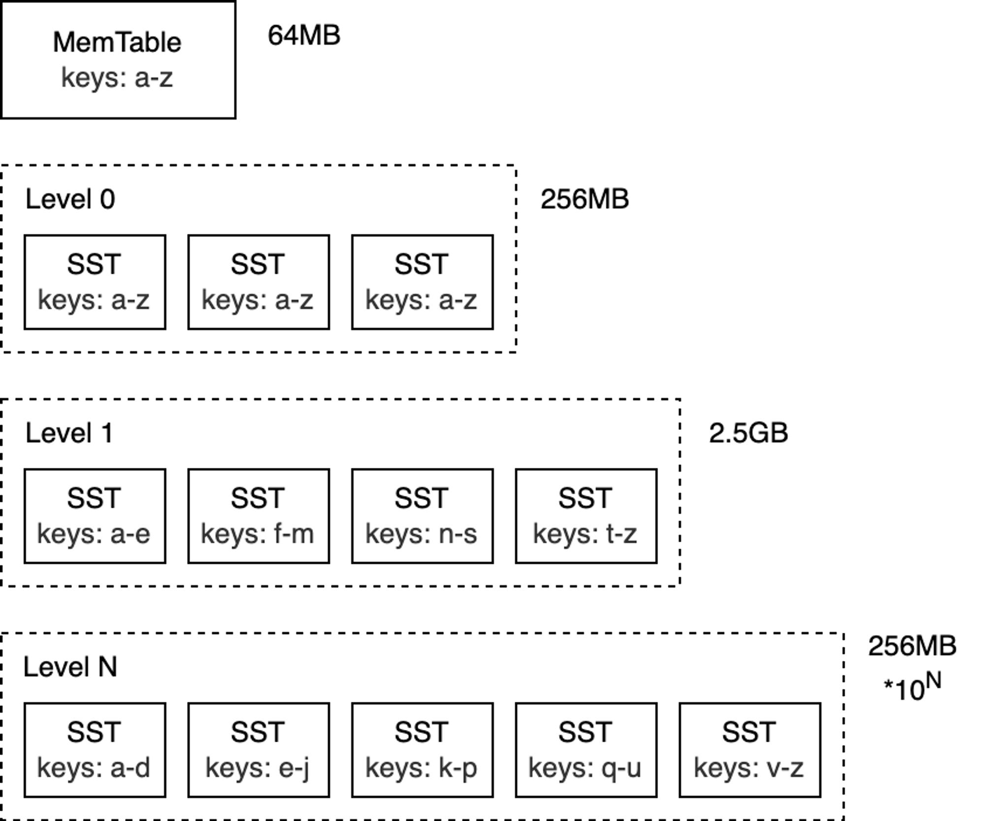
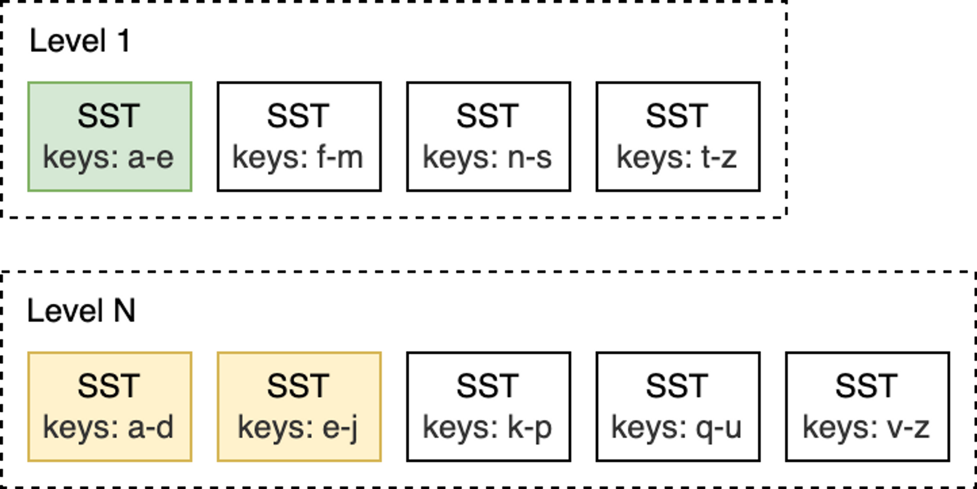
The core data structure of RocksDB is called the Log-Structured Merge-Tree (LSM-Tree). It is a tree-like data structure composed of multiple levels, with data sorted by key at each level. The LSM-Tree was primarily designed to handle write-intensive workloads and was introduced in the 1996 paper The Log-Structured Merge-Tree (LSM-Tree).
The top level of the LSM-Tree resides in memory and contains the most recently written data. The other lower levels store data on disk, with levels numbered from 0 to N. Level 0 (L0) stores data that has been moved from memory to disk, while Level 1 and below store older data. Typically, each subsequent level is an order of magnitude larger than the previous one in terms of data volume. When a level becomes too large, it is merged into the next level.
 blog_how-rocksdb-works_rocksdb-lsm.png
Note: Although this article mainly discusses RocksDB, the LSM-Tree concepts apply to most databases that use this technology under the hood (e.g., Bigtable, HBase, Cassandra, ScyllaDB, LevelDB, and MongoDB WiredTiger).
To better understand how the LSM-Tree works, we will focus on analyzing its write and read paths.
Write Path
MemTable
The top layer of the LSM-Tree is called the MemTable. The MemTable is an in-memory buffer that caches key-value pairs before they are written to disk. All insert and update operations go through the MemTable. This also includes delete operations: however, in RocksDB, key-value pairs are not modified in place; instead, deletes are performed by inserting tombstone records.
The MemTable has a configurable byte size limit. When a MemTable becomes full, it is switched to a new MemTable, and the original MemTable becomes immutable.
Note: The default size of a MemTable is 64 MB.
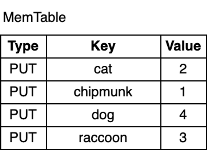
Now, let’s write some keys into the database:
1 | db.put("chipmunk", "1") |
 how-rocksdb-works-memtable.png
As shown in the figure above, the key-value pairs in the MemTable are sorted by key. Although chipmunk was inserted first, because the MemTable is sorted by key, chipmunk comes after cat. This ordering is essential for range scans, and as I will explain later, it also makes certain operations more efficient.
Write-Ahead Log
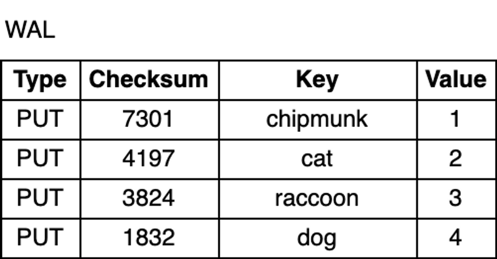
Whether due to an unexpected process crash or a planned restart, data in memory is lost. To prevent data loss and ensure durability, in addition to the MemTable, RocksDB writes all updates to a Write-Ahead Log (WAL) on disk. This way, after a restart, the database can replay the log to recover the original state of the MemTable.
The WAL is an append-only file containing a sequence of change records. Each record includes the key-value pair, the record type (Put / Merge / Delete), and a checksum. Unlike the MemTable, records in the WAL are not sorted by key; instead, they are appended in the order the requests arrive.
 how-rocksdb-works-wal.png
Flush
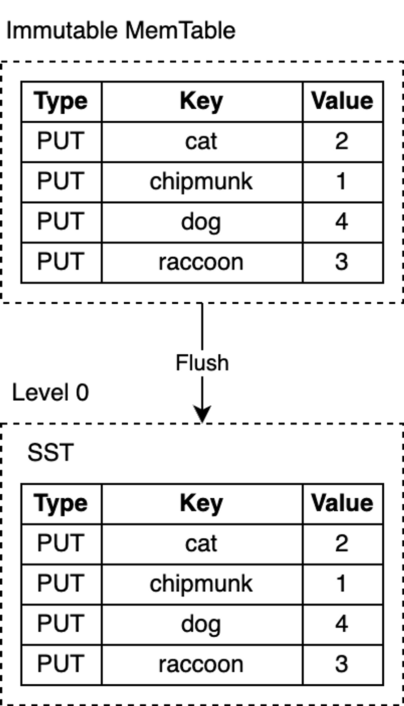
RocksDB uses a dedicated background thread to periodically persist immutable MemTables from memory to disk. Once a flush is complete, the immutable MemTable and the corresponding WAL are discarded. RocksDB then starts writing to a new WAL and MemTable. Each flush produces a new SST file at the L0 level. Once this file is written to disk, it is never modified again.
RocksDB’s MemTable is implemented based on a skip list by default. This data structure is a linked list with additional sampling layers, enabling fast, ordered queries and insertions. The ordering makes flushing the MemTable more efficient, because key-value pairs can be directly iterated in order and written sequentially to disk. Turning random writes into sequential writes is one of the core designs of the LSM-Tree.
 how-rocksdb-works-flush.png
Note: RocksDB is highly configurable, so you can configure alternative implementations for the MemTable, as is the case for most components in RocksDB. In some other LSM-based databases, using self-balancing binary search trees to implement the MemTable is not uncommon.
SST
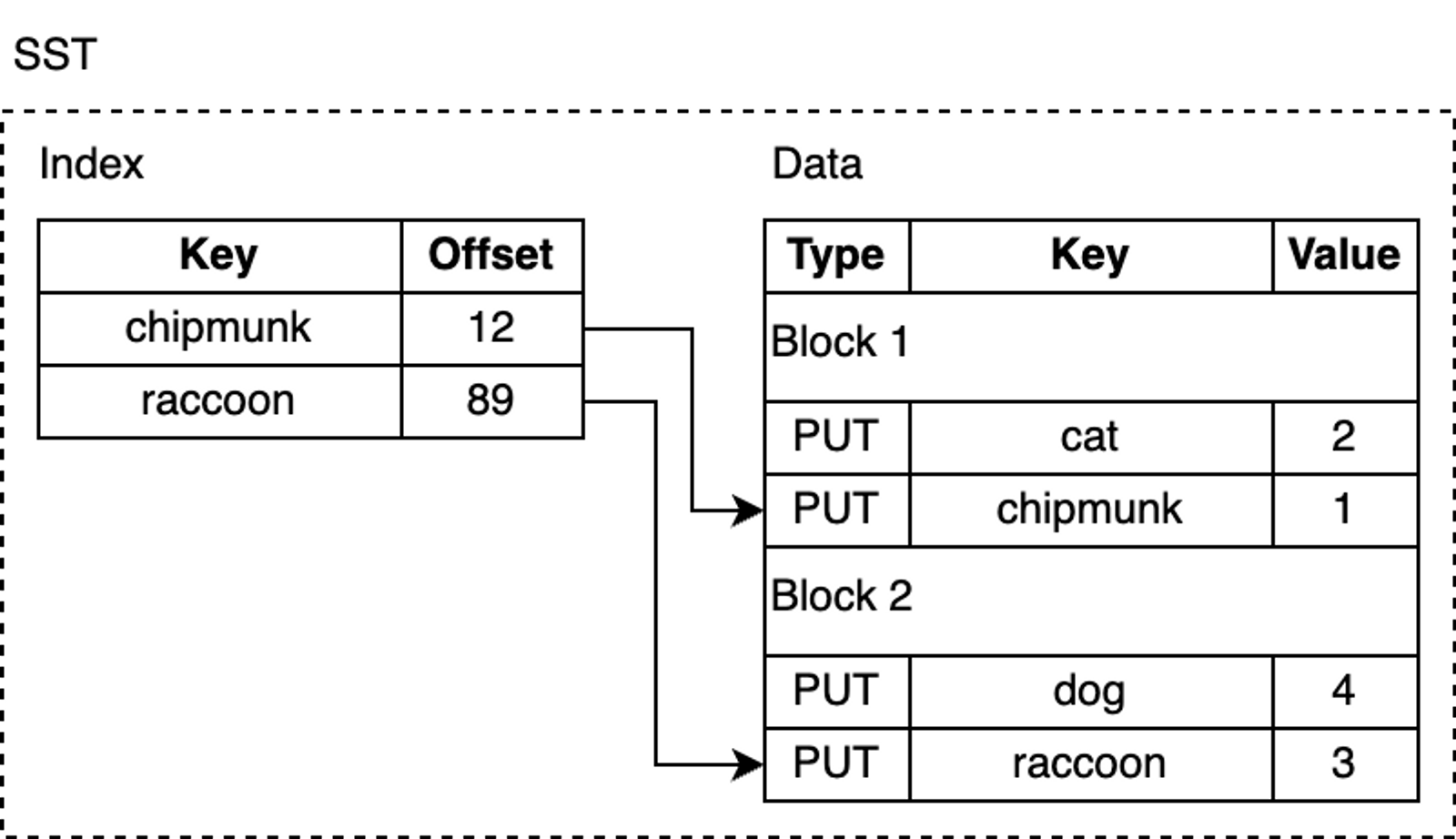
SST files contain key-value pairs flushed from the MemTable and are stored in a query-friendly data format. SST stands for Static Sorted Table (also known as Sorted String Table in other databases). It is a block-based file format that splits data into fixed-size blocks (default 4KB) for storage. RocksDB supports various compression algorithms for compressing SST files, such as Zlib, BZ2, Snappy, LZ4, or ZSTD. Similar to WAL records, each data block contains a checksum for detecting data corruption. Every time data is read from disk, RocksDB validates it using these checksums.
An SST file consists of several parts: first, the data section, which contains a sequence of sorted key-value pairs. The sortedness of keys allows for delta encoding—that is, for adjacent keys, we can store only the difference rather than the entire key.
Although key-value pairs in an SST are sorted, we cannot always perform binary search, especially after data blocks are compressed, which makes lookups inefficient. RocksDB uses an index to optimize queries, stored in an index block immediately following the data blocks. The index maps the last key of each data block to its corresponding offset on disk. Likewise, the keys in the index are sorted, so we can quickly find a key via binary search.
 how-rocksdb-works-sstable.png
For example, when looking up lynx, the index tells us that this key-value pair is likely in block 2, because lexicographically, lynx comes after chipmunk but before raccoon.
However, lynx may not actually exist in the SST file, but we still need to load the block from disk to search for it. RocksDB supports enabling a Bloom filter, a space-efficient probabilistic data structure that can be used to test whether an element is in a set. The Bloom filter is stored in the filter section of the SST file, so that we can quickly determine whether a key is definitely not in the SST (thus avoiding the cost of touching data blocks on disk).
In addition, SST files have several other less interesting parts, such as the metadata section.
Compaction
So far, we have described a fully functional key-value storage engine. But if deployed to production as-is, there are some problems: space amplification and read amplification. Space amplification is the ratio of the actual disk space used to store data to the logical size of the data. For example, if a database requires 2 MB of disk space to store 1 MB of logical key-value pairs, its space amplification is 2. Similarly, read amplification measures the actual number of I/O operations the system performs for a single logical read operation. As a small exercise, you can try to deduce what write amplification is.
Now, let’s add more keys to the database and delete some of them:
1 | db.delete("chipmunk") |
 blog_how-rocksdb-works_rocksdb-compaction1.png
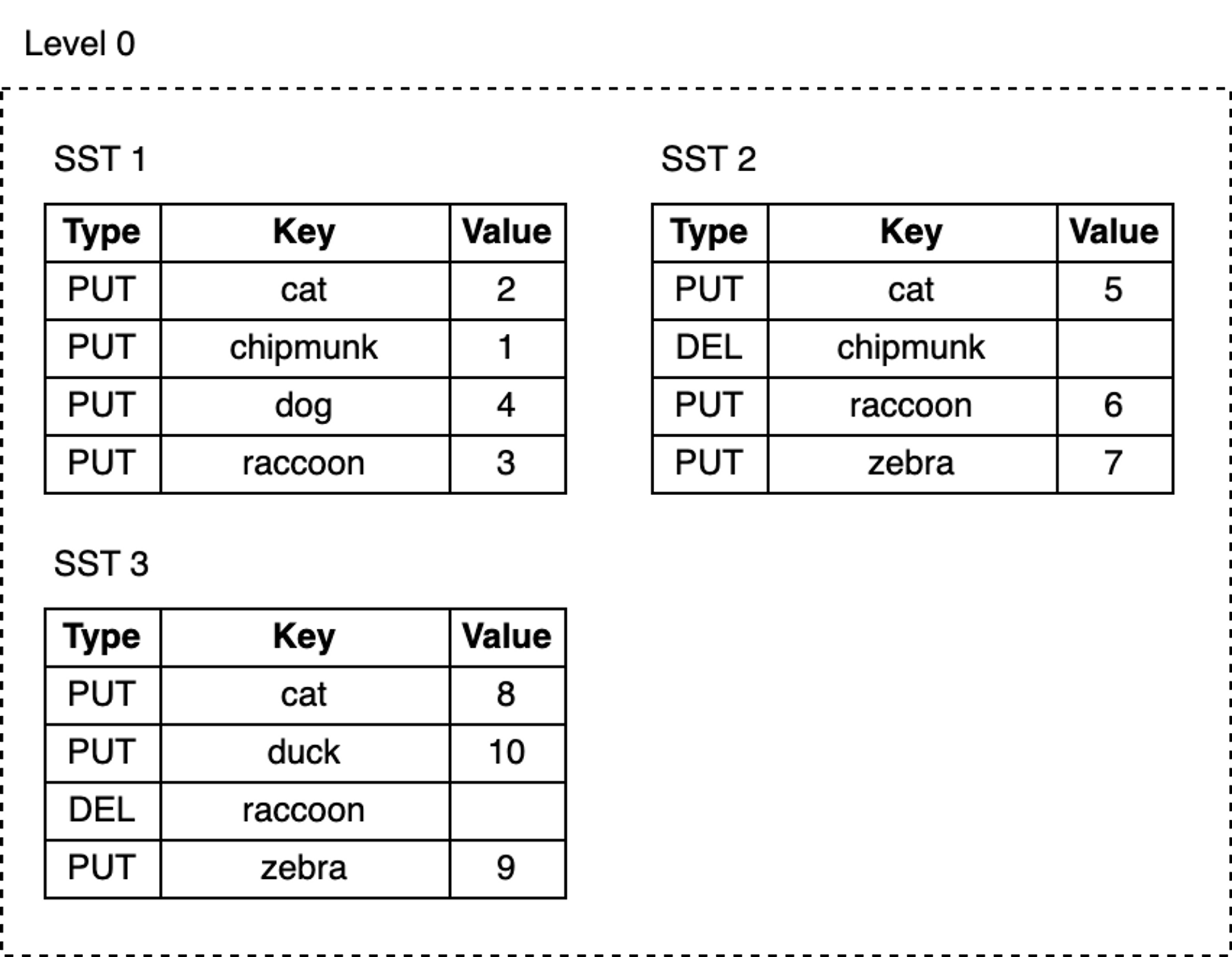
As we keep writing, MemTables are continuously flushed to disk, and the number of SST files at L0 grows:
- Space occupied by deleted or updated keys is never reclaimed. For example, the three update records for the key
catare in SST1, SST2, and SST3 respectively, whilechipmunkhas one update record in SST1 and one delete record in SST2. These obsolete records still occupy extra disk space. - As the number of SST files at L0 increases, reads become slower. Every lookup must check all SST files one by one.
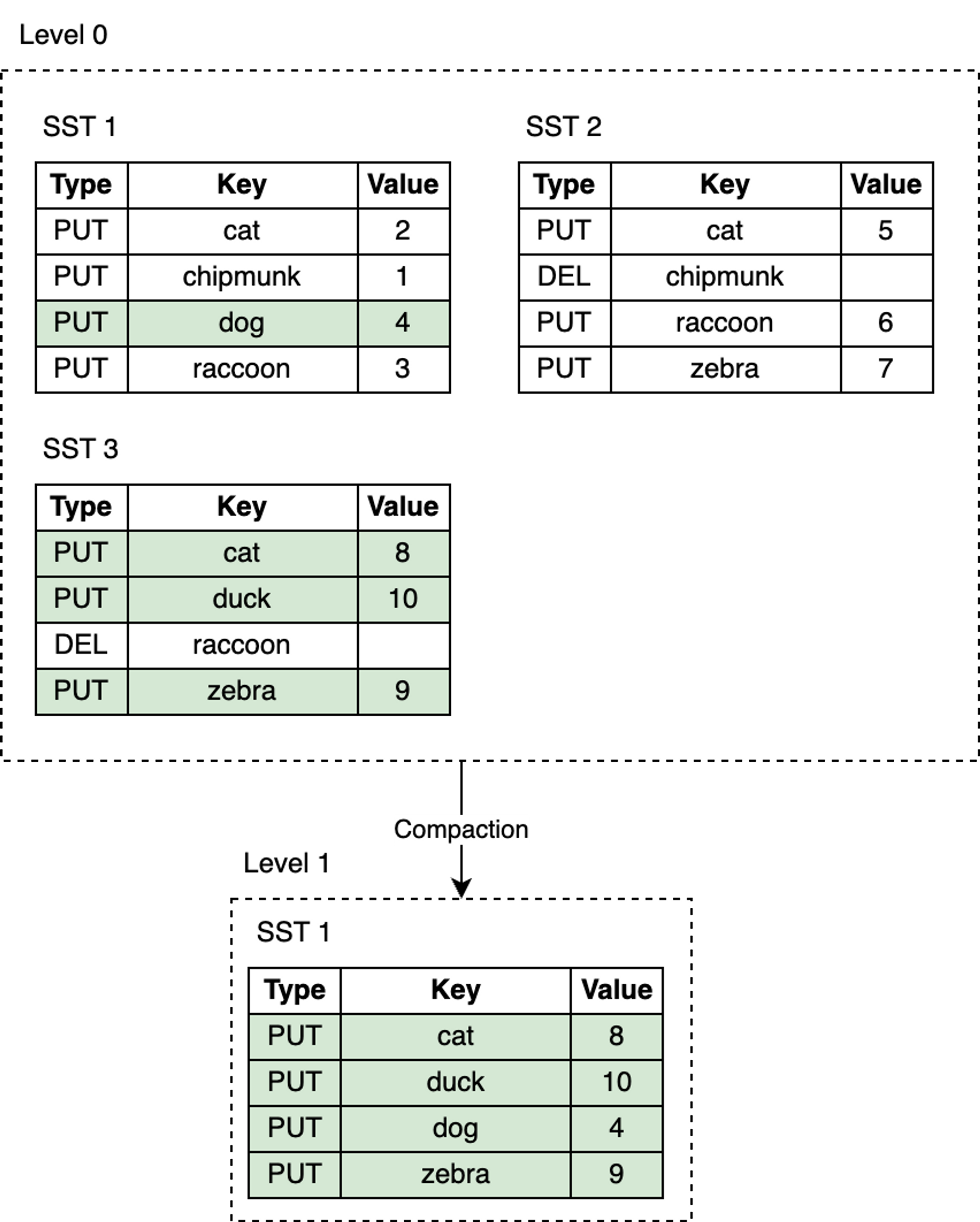
RocksDB introduces the compaction mechanism to reduce space amplification and read amplification, at the cost of higher write amplification. Compaction merges SST files from one level with SST files in the next level, discarding invalid keys that have been deleted or overwritten during this process. Compaction runs in a dedicated background thread pool, ensuring that RocksDB can continue to process user read and write requests while compaction is ongoing.
 blog_how-rocksdb-works_rocksdb-compaction2.png
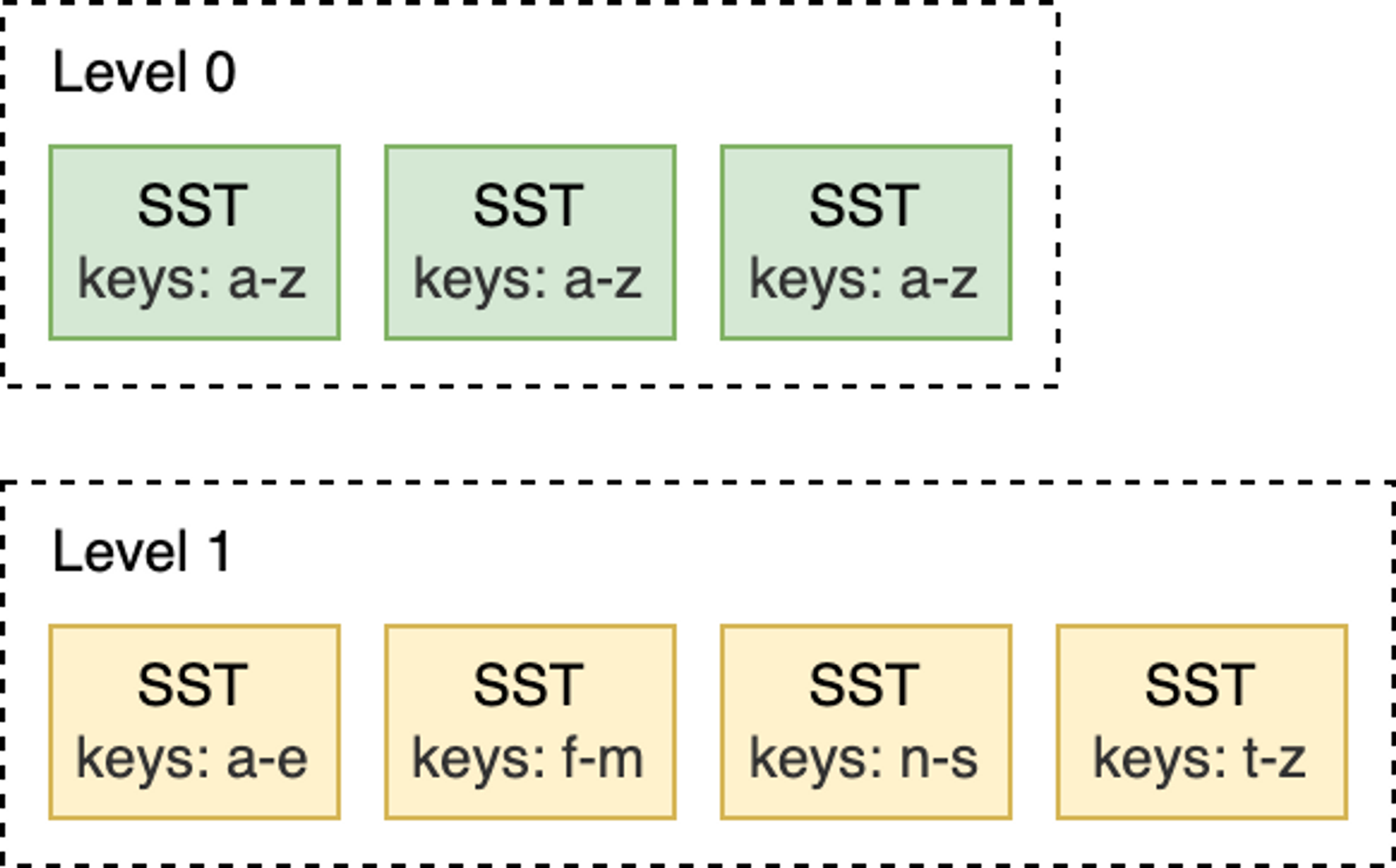
Leveled Compaction is the default compaction strategy in RocksDB. With Leveled Compaction, different SST files at L0 may have overlapping key ranges. Level 1 and below are organized as a sequence of multiple SST files, ensuring that all SST files within the same level have non-overlapping key ranges and are sorted among themselves. During compaction, SST files from one level are selectively merged with SST files in the next level whose key ranges overlap.
For example, as shown in the figure below, when compacting from L0 to L1, if the input file at L0 covers the entire key range, then all files at L0 and L1 need to be compacted.
 blog_how-rocksdb-works_rocksdb-compaction3.png
In contrast, in the L1-to-L2 compaction shown below, the input file at L1 overlaps with only two SST files at L2, so only those files need to be compacted.
 blog_how-rocksdb-works_rocksdb-compaction4.png
When the number of SST files at L0 reaches a certain threshold (default is 4), compaction is triggered. For Level 1 and below, compaction is triggered when the total size of SST files in the entire level exceeds the configured target size. When this happens, it may trigger an L1-to-L2 compaction. Thus, an L0-to-L1 compaction may trigger a cascading compaction all the way down to the lowest level. After compaction completes, RocksDB updates its metadata and deletes the compacted files from disk.
Note: RocksDB provides different compaction strategies to trade off between space, read amplification, and write amplification.
At this point, do you still remember that I mentioned earlier that keys in SST files are sorted? This sortedness allows the use of the K-way merge algorithm to gradually merge multiple SST files. K-way merge is a generalization of two-way merge, working similarly to the merge phase of merge sort.
Read Path
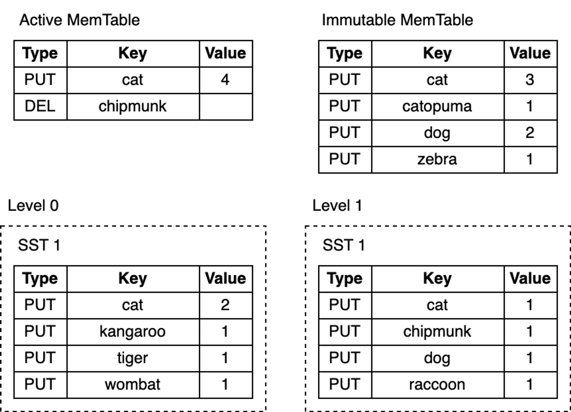
With immutable SST files persisted on disk, the read path is much simpler than the write path. To find a key, you simply traverse the LSM-Tree from top to bottom. Start from the MemTable, descend to L0, and continue searching lower levels until the key is found or all SST files have been checked.
Here are the lookup steps:
- Search the MemTable.
- Search the immutable MemTables.
- Search all SST files in the most recently flushed L0 level.
- For Level 1 and below, first find the single SST file that may contain the key, then search within that file.
Searching an SST file involves:
- (Optional) Probe the Bloom filter.
- Look up the index to find the location of the block that may contain the key.
- Read the block and attempt to find the key within it.
That’s all there is to it! Take a look at this LSM-Tree:
 blog_how-rocksdb-works_rocksdb-lookup.png
Depending on the specific key being looked up, the search may terminate early at any of the steps above. For example, after searching the MemTable, lookups for the keys “cat” or “chipmunk” will end immediately. Looking up “raccoon” requires searching down to L1, while looking up the non-existent “manul” requires searching the entire tree.
Merge
RocksDB also provides a feature that involves both the read and write paths: the merge operation. Suppose you store a list of integers in the database and occasionally need to extend it. To modify the list, you need to read its existing value from the database, update the list in memory, and finally write the updated value back to the database.
The entire sequence of operations above is known as a “Read-Modify-Write” cycle:
1 | db = open_db(path) |
The above approach achieves the goal, but it has some drawbacks:
- Not thread-safe—two different threads trying to update the same key, interleaving their execution, can lead to lost updates.
- Write amplification—as values become larger, the cost of updates also increases. For example, appending a single integer to a list of 100 integers requires reading 100 integers and writing 101 integers back.
In addition to Put and Delete write operations, RocksDB supports a third write operation: Merge. The Merge operation requires a Merge Operator—a user-defined function responsible for combining incremental updates into a single value:
1 | funcmerge_operator(existing_val, updates) { |
The merge_operator above combines the incremental updates passed to Merge calls into a single value. When Merge is called, RocksDB only inserts the incremental updates into the MemTable and WAL. Later, during flush and compaction, RocksDB calls merge_operator() to merge multiple updates into a single update or a single value when conditions permit. When users call Get or perform scan reads, if any pending merge updates are found, merge_operator is also called to return a merged value to the user.
Merge is very suitable for write-intensive scenarios where existing values need to be continuously updated with small changes. So, what is the cost? Reads become more expensive—the merged value at read time is not written back. Queries for that key need to perform the same merge process over and over again until flush and compaction are triggered. Like other parts of RocksDB, we can optimize read behavior by limiting the number of merge operands in the MemTable and reducing the number of SST files in L0.
Challenges
If your application is very sensitive to performance, the biggest challenge of using RocksDB is the need to tune its configuration for specific workloads. RocksDB provides a vast number of configuration options, but adjusting them properly usually requires understanding the internal principles of the database and delving into the RocksDB source code:
“Unfortunately, tuning RocksDB is not easy. Even as RocksDB developers, we do not fully understand the impact of every configuration change. If you want to fully tune for your workload, we recommend experimenting and benchmarking, and always keeping an eye on the three amplification factors.”
– RocksDB Official Tuning Guide
Summary
Writing a production-grade KV store from scratch is extremely difficult:
- Hardware and operating systems can lose or corrupt data at any time.
- Performance optimization requires a significant time investment.
RocksDB solves both of the above problems, allowing you to focus on implementing upper-layer business logic. This also makes RocksDB an excellent building block for constructing databases.
This article is from my paid newsletter column. The preliminary plan includes the following series:
- Graph Database 101 Series
- Learn a Bit of Databases Every Day Series
- Great Articles Recommendation Series
- Reading Notes Series
- Data-Intensive Paper Reading Series
I will guarantee at least two updates per week. For subscription details, see the column introduction. Welcome subscriptions and support from friends who enjoy my articles, to motivate me to produce more high-quality content.