The Theoretical Foundation of Spark — RDD

Overview

RDD, whose full name is Resilient Distributed Dataset, is an abstraction over dataset shapes. Based on this abstraction, users can execute a series of computations on a cluster without persisting intermediate results to disk. This was exactly a major pain point of the earlier MapReduce abstraction — every step required disk writes, leading to high unnecessary overhead.

For distributed systems, fault tolerance support is essential. To support fault tolerance, RDD only supports coarse-grained transformations. That is, the input dataset is immutable (or read-only), and each computation produces a new output. Fine-grained update operations on a dataset are not supported. This constraint greatly simplifies fault tolerance support and can satisfy a large class of computation needs.

When first encountering the concept of RDD, it was somewhat difficult to understand why the abstraction should be centered around datasets. As I delved deeper, I realized that a consistent abstraction over datasets is precisely the essence that enables the existence and optimization of computational pipelines. After defining the basic properties of a dataset (immutability, partitioning, dependencies, placement, etc.), various high-level operators can be applied on top of it to build a DAG execution engine and perform appropriate optimizations. From this perspective, RDD is truly an elegant design.

As usual, let me summarize the main design points of the RDD paper:

1. Explicit abstraction. Datasets used in computations are explicitly abstracted, with their interfaces and properties defined. Thanks to the unified dataset abstraction, different computation processes can be combined for unified DAG scheduling.
2. Memory-based. Compared to MapReduce where intermediate results must be written to disk, RDD significantly reduces the latency of individual operator computation and the loading latency between different operators by keeping results in memory.
3. Narrow vs. wide dependencies. When performing DAG scheduling, the concepts of narrow and wide dependencies are defined and used for stage division and scheduling optimization.
4. Lineage-based fault tolerance. Error recovery mainly relies on computing from the lineage graph rather than maintaining redundant backups, because memory is limited after all — we trade computation for storage.
5. Interactive queries. The Scala interpreter was modified to enable interactive querying of large datasets based on multi-machine memory, thereby supporting higher-level query languages like SQL.

Author: Muniao’s Notes https://www.qtmuniao.com, please indicate the source when reprinting

Introduction

Dryad and MapReduce are already popular big data analysis tools. They provide users with some high-level operators without needing to worry about the underlying distributed and fault-tolerance details. However, they both lack an abstraction for distributed memory; different computation processes can only be coupled through external storage: the predecessor task writes its results to external storage, and the successor task loads them into memory as input before continuing with the successor computation. Such a design has two major drawbacks: poor reusability and high latency. This is extremely unfriendly to machine learning algorithms that require iterative computation (such as PageRank, K-Means, LR, which need data reuse); it is also a disaster for random interactive queries (which require low latency). Because most of the time is spent on data backup, disk I/O, and data serialization.

Before RDD, there had been many attempts in the industry to solve the data reuse problem. These include iterative graph computing systems that keep intermediate results in memory — Pregel, and HaLoop, which strings together multiple MapReduce jobs and caches loop invariants. However, these systems only support restricted computation models (such as MR) and only perform implicit[1] data reuse. How to achieve more general data reuse to support more complex query computation remains a difficult problem.

RDD was designed to solve this problem — an efficient data structure abstraction for data reuse. RDD supports data fault tolerance and data parallelism; on top of this, it allows users to leverage multi-machine memory, control data partitioning, and construct a series of computation processes. Thereby solving the data reuse needs of many applications with continuous computation processes.

One of the more difficult design aspects is how to perform efficient fault tolerance for in-memory data. Some existing cluster-memory-based systems, such as distributed key-value stores, shared memory, and Piccolo, provide a mutable dataset abstraction that allows fine-grained modifications. To support fault tolerance on top of this abstraction, data replication across machines or operation log backups are required. These operations would cause large amounts of data transfer between machines. Since network bandwidth is much slower than RAM, this undermines the advantage of distributed memory utilization.

In contrast, RDD only provides coarse-grained computation interfaces based on entire datasets, meaning all entries in a dataset are subjected to the same operation. This way, for fault tolerance, we only need to back up each operation rather than the data itself (because updates are performed on the whole dataset); when recovering from errors in a partition, we only need to start from the original dataset and recompute sequentially.

At first glance, this computation abstraction seems very limited, but it actually satisfies a large class of existing cluster computation needs, including MR, DryadLINQ, SQL, Pregel, and HaLoop. It can also satisfy some other computation needs, such as interactive computation. Spark, the implementation system of RDD, provides high-level operators similar to DryadLINQ and should be the first to provide interactive cluster computation interfaces.

RDD

This section first gives a detailed definition of RDD, then introduces the operation interfaces for RDD in Spark, compares RDD with shared memory abstractions that provide fine-grained update interfaces, and finally discusses the limitations of RDD.

RDD Abstraction

RDD is a partitioned, read-only abstraction over a set of data records. RDDs can only be obtained through deterministic computations on persistent storage or other RDDs; such computations are called transformations. Common transformation operators include map, filter, and join.

Instead of constantly taking checkpoints for fault tolerance, RDD records the path of changes from the initial external storage dataset, which is its lineage. Theoretically, all RDDs can be rebuilt from external storage according to the lineage graph after an error occurs. Generally, the reconstruction granularity is the partition rather than the entire dataset — first because the cost is smaller, and second because different partitions may be on different machines.

Users can control two aspects of RDDs: persistence and partitioning. For the former, if some RDDs need to be reused, users can instruct the system to persist them according to some strategy. For the latter, users can customize partition routing functions to route records in the dataset to different partitions based on some key. For example, when performing a join operation, the datasets to be joined can be partitioned according to the same strategy for parallel join.

Spark Programming Interface

Spark provides interfaces for operating on RDDs by exposing operators integrated with the programming language. RDDs appear as classes in the programming language, and RDD operators are functions that act on these classes. Previous systems such as DryadLINQ and FlumeJava also used a similar form.

When using RDDs, users first load data from persistent storage into memory through transformations (such as map or filter), then can apply any series of transformations supported by the system to the RDDs, and finally use actions to persist the RDDs back to external storage or return control to the user. Like DryadLINQ, this load-transform-persist process is declarative (or lazy[2]): Spark uses the execution engine to perform execution optimization (such as parallelization and pipelining) after obtaining the entire topology.

Another important interface is persist, which allows users to tell the system which RDDs need to be persisted, how to persist them (local disk or cross-machine storage), and if multiple RDDs need to be persisted, how to determine priority. Spark saves RDDs in memory by default; if memory is insufficient, it will spill data to disk according to user configuration.

An Example

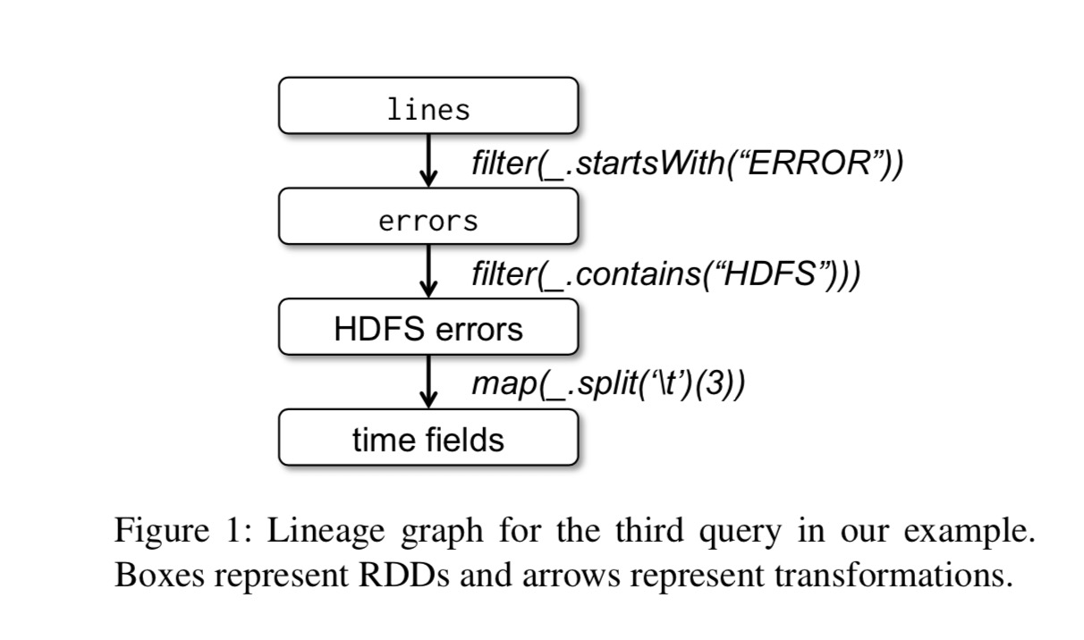
Suppose we want to find error entries in a log file stored on HDFS and analyze specific entries containing the keyword “hdfs”. Using the Spark interface and implementing it in Scala, the code is as follows:

lines = spark.textFile("hdfs://...")
errors = lines.filter(_.startsWith("ERROR"))
errors.persist()

// Return the time fields of errors mentioning
// HDFS as an array (assuming time is field
// number 3 in a tab-separated format):
errors.filter(_.contains("HDFS"))
      .map(_.split('\t')(3))
      .collect()

The first line defines an RDD based on a file on HDFS (each line as an entry in the collection). The second line generates a new RDD through the filter transformation. The third line requests Spark to cache its results. The last line is a chain of operations ending with a collect action, obtaining the various fields of all lines containing the HDFS keyword.

Its computation lineage graph is as follows:

rdd-example-lineage.jpg

There are two points to note:

1. No actual computation occurs until the action (Action) collect is encountered.
2. Intermediate results are not saved during chained operations;

Since the third line caches results in memory, other actions can also be based on this. For example, counting error entries containing the ‘MySQL’ keyword:

// Count errors mentioning MySQL:
errors.filter(_.contains("MySQL")).count()

Advantages of the RDD Model

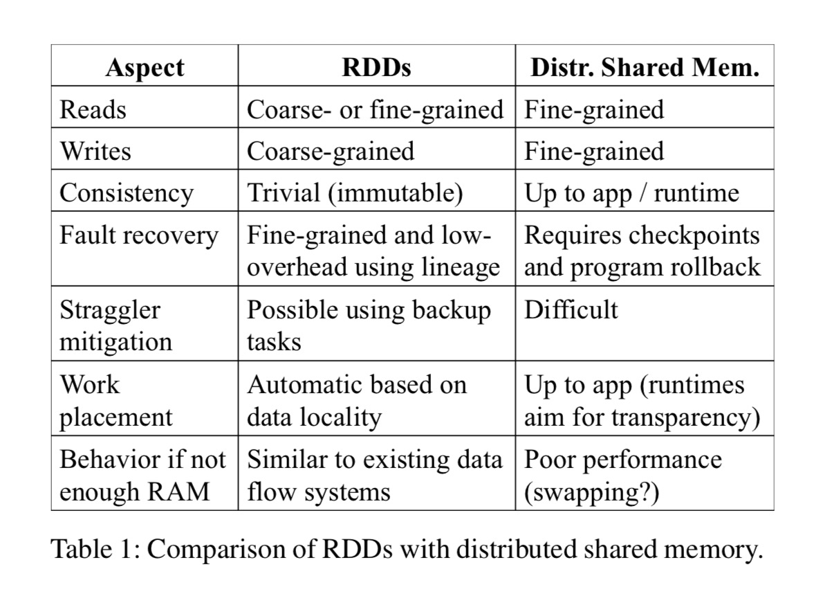
To understand the benefits brought by RDD, consider the following table, which compares RDD with DSM (Distributed Shared Memory) in detail. DSM here is a very broad abstraction, including not only general memory sharing systems but also other frameworks that support fine-grained state updates, such as Piccolo and distributed databases.

rdd-compare-dsm-table.jpg

First, the main difference between DSM and RDD is that DSM supports fine-grained updates to datasets. That is, updates can be made to arbitrary memory locations. RDD gives up this capability and only allows batch data writes, thereby improving fault tolerance efficiency:

1. Using lineage to recover data on demand, rather than periodic snapshots, reduces unnecessary overhead.
2. Each partition can be recovered independently after an error, without rebuilding the entire dataset.

Second, the immutable nature of RDDs allows the system to relatively easily migrate certain computations. For example, some straggler tasks in MR can be conveniently migrated to other compute nodes because their input data will definitely not change, so consistency issues need not be considered.

Finally, two more benefits are worth mentioning:

1. Because only batch computation is supported, the scheduling system can better exploit data locality to speed up computation.
2. If cluster memory is insufficient, as long as the data supports iteration, it can be loaded into memory in batches for computation, or results can be spilled to external storage in batches. In this way, it can provide very elegant degradation when memory is insufficient without much performance loss.

Scenarios Where RDD Is Not Suitable

As mentioned above, RDD is suitable for coarse-grained transformation abstractions that apply unified processing to entire datasets. Correspondingly, it is not suitable for datasets that require fine-grained, asynchronous updates to data. For example, web applications, or web crawlers, etc. For these application types, traditional snapshot + operation log fault tolerance methods may be more suitable, such as databases RAMCloud, Percolator, and Piccolo. RDD targets batch analytical applications, leaving the needs of these asynchronous applications to specialized systems.

Spark Programming Interface

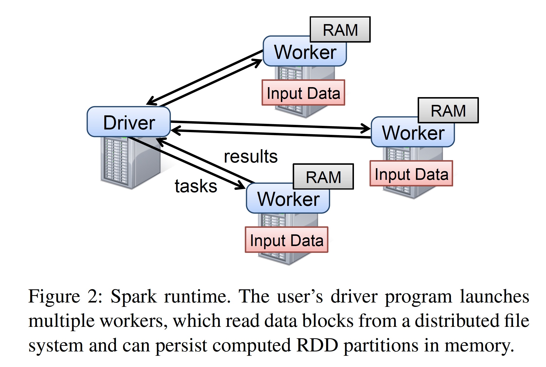
Spark uses the Scala language as the interface for the RDD abstraction because Scala balances precision (its functional semantics are suitable for interactive scenarios) with efficiency (using static types). Of course, for RDD itself, it is not limited to any particular language expression. Below, we explain in detail how Spark executes user code from two aspects: execution flow and code distribution.

rdd-spark-runtime.jpg

Developers use the libraries provided by Spark to write driver programs to use Spark. The driver program defines one or more RDDs and applies various transformations to them. The libraries provided by Spark connect to the Spark cluster, generate a computation topology, distribute the topology to multiple workers for execution, and record the lineage of transformations. These workers are long-running processes distributed across machines in the Spark cluster; they store partitions of RDDs generated during computation in memory.

As in the previous example, developers need to pass functions as arguments to Spark operators such as map. Spark serializes these functions (or closures) into Java objects and distributes them to execution nodes for loading. Variables involved in closures are treated as field values of the generated objects. RDDs themselves are packaged as statically typed parameters for passing. Since Scala supports type inference, most examples omit the RDD data type.

Although the Scala RDD interface exposed by Spark appears conceptually simple, there are some very dirty corners in its actual implementation, such as Scala closures requiring reflection, and trying to avoid modifying the Scala interpreter.

RDD Operations in Spark

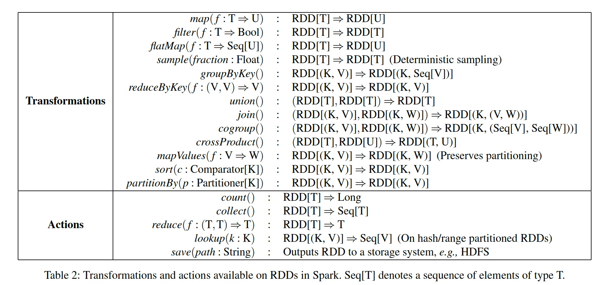
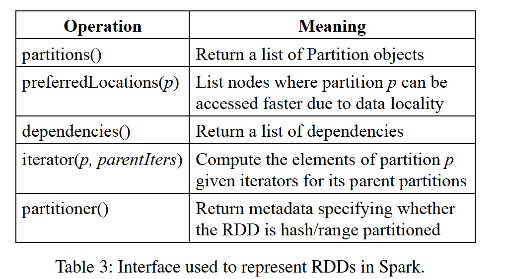
The following table lists the RDD operations supported in Spark. As mentioned earlier, transformations are lazy operators that generate new RDDs, while actions are operators that trigger scheduling; they return a result or write data to external storage.

rdd-operations-table.jpg

Points to note:

1. Some operations, such as join, require the operand RDDs to be key-value pairs.
2. map is a one-to-one mapping, while flatMap is a one-to-one or one-to-many mapping similar to that in MapReduce.
3. save persists an RDD.
4. groupByKey, reduceByKey, and sort all cause re-hashing or reordering across different partitions of an RDD.

Representation of RDDs

One difficulty in providing the RDD abstraction is how to efficiently track lineage while providing rich transformation support. We ultimately chose a graph-based scheduling model, decoupling scheduling from operators. Thereby, operator support can be conveniently increased without changing the scheduling module logic. Specifically, the core components of the RDD abstraction mainly consist of the following five parts:

1. Partition set. Partitions are the smallest constituent units of each RDD.
2. Dependency set. Mainly the parent-child dependency relationships between RDDs.
3. Compute function. The transformation function applied to partitions, which can compute a child partition from several parent partitions.
4. Partition scheme. Whether the RDD is partitioned based on hash sharding or direct splitting.
5. Data placement. Knowing partition placement locations enables computation optimization.

RDD Abstraction Interface Composition

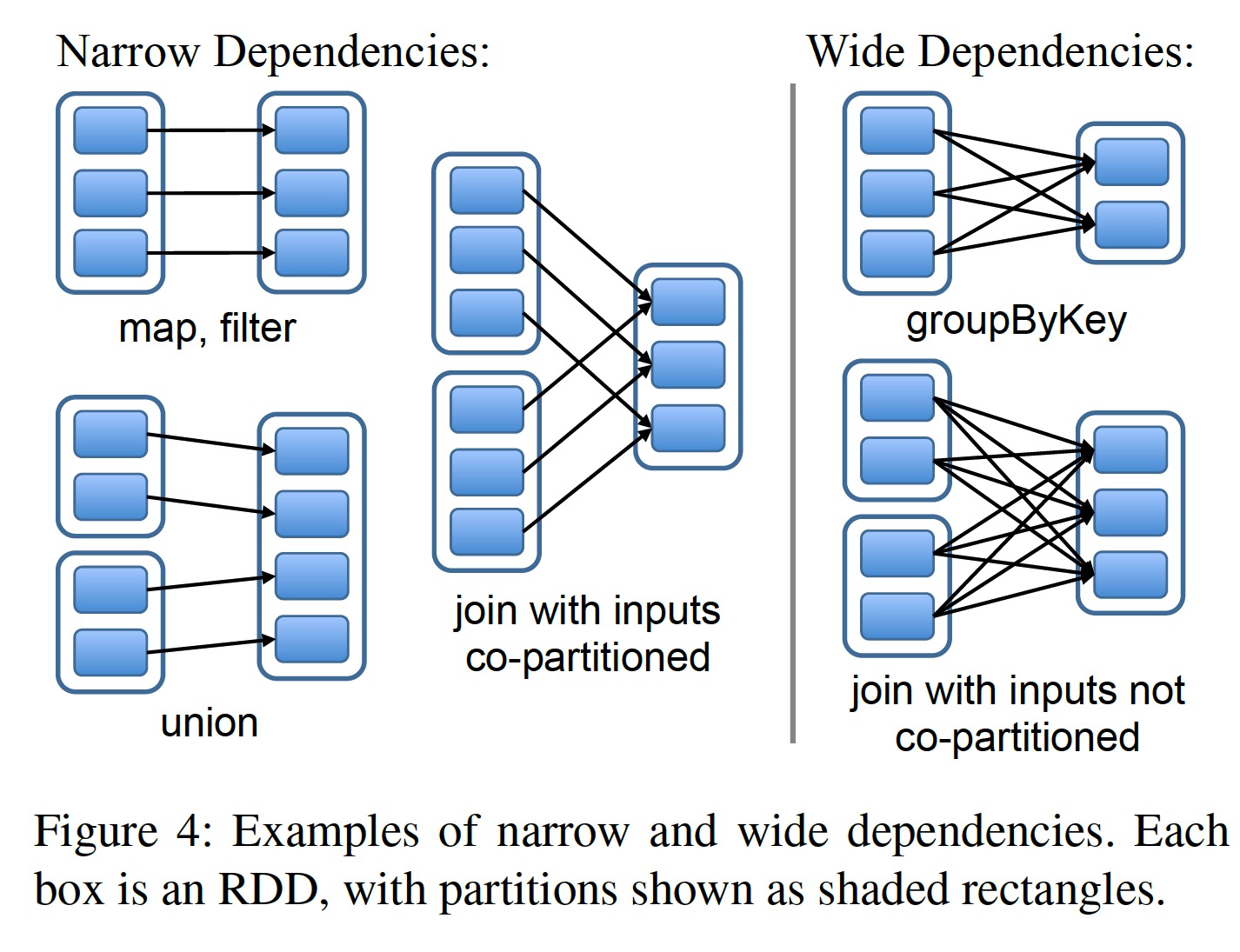
One of the most interesting points in the RDD interface design is how to reduce the dependency relationships between RDDs. It was ultimately discovered that all dependencies can be categorized into two types:

1. Narrow dependencies: A partition of the parent RDD is depended upon by at most one partition of the child RDD, such as map.
2. Wide dependencies: A partition of the parent RDD may be depended upon by multiple partitions of the child RDD, such as join.

Wide and Narrow Dependencies

The main reasons for this categorization are two-fold.

Scheduling optimization. For narrow dependencies, pipelined scheduling can be performed between partitions: a partition that has completed a narrow dependency operator (such as map) does not need to wait for other partitions and can directly proceed to the next narrow dependency operator (such as filter). In contrast, wide dependencies require all partitions of the parent RDD to be ready and transferred across nodes before computation can proceed, similar to the shuffle in MapReduce.

Data recovery. When a partition encounters an error or is lost, recovery for narrow dependencies is more efficient. Because fewer parent partitions are involved, and recovery can be performed in parallel. For wide dependencies, due to complex dependencies (as shown in the figure above, each partition of the child RDD depends on all partitions of the parent RDD), the loss of one partition may trigger a full recomputation.

This design that decouples scheduling from operators greatly simplifies the implementation of transformations; most transformations can be implemented in about 20 lines of code. Since there is no need to understand scheduling details, anyone can quickly get started implementing a new transformation. A few examples:

HDFS file: The partitions function returns all blocks of the HDFS file, with each block treated as a partition. preferredLocations returns the location of each block, and Iterator reads each block.

map: Calling map on any RDD returns a MappedRDD object, whose partitions function and preferredLocations are consistent with the parent RDD. For iterator, we only need to apply the function passed to the map operator to each partition of the parent RDD in turn.

union: Calling union on two RDDs returns a new RDD, each partition of which is computed from the corresponding two parent RDDs through narrow dependencies.

sample: The sampling function is largely consistent with map. However, this function saves a random seed for each partition to decide whether each record of the parent RDD is retained.

join: Calling join on two RDDs may result in two narrow dependencies (if their partitions are both hashed by the key to be joined), two wide dependencies, or mixed dependencies. In each case, the child RDD will have a partitioner function, either inherited from the parent partition or using the default hash partition function.

Implementation

The initial version of Spark (mentioned in the paper) consisted of only 14,000 lines of Scala code, managed resource allocation by Mesos, could share resources with the Hadoop ecosystem, and loaded data from Hadoop/HBase. Regarding Spark’s implementation, there are several points worth discussing: Job scheduling, interactive interpreter, memory management, and checkpointing.

Job Scheduling

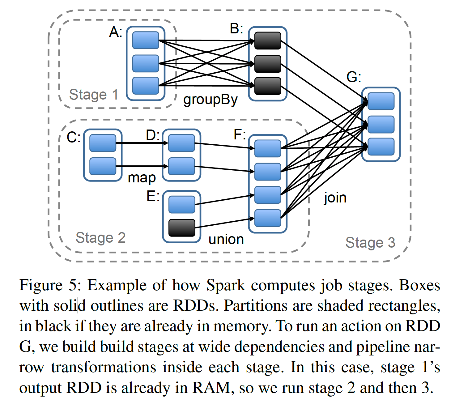
Spark’s scheduling design relies on the RDD abstraction mentioned in the previous section. Its scheduling strategy is somewhat similar to Dryad’s but not exactly the same. When a user calls an Action-type operator (such as count, save, etc.) on an RDD, the scheduler generates a computation topology based on the order in which operators are called in the user code. We treat each RDD before and after a transformation as a node, and the dependency/parent-child relationships between RDDs generated by operators as edges, thereby forming a directed acyclic graph (DAG). To reduce transfer, the scheduler merges several consecutive computations into a stage. The criterion for stage merging is whether a shuffle is needed, that is, whether it is a wide dependency. This forms a new, more streamlined DAG composed of stages.

RDD Stage Division

After that, the scheduler starts from the target RDD and traverses forward along the edges in the DAG graph, computing each partition that is not in memory. If the partition to be computed is already in memory, the result is directly used, as shown in the figure above.

Then, the scheduler schedules tasks to locations close to the partitions of their dependent RDDs:

1. If a partition is in the memory of a node, the task is scheduled to that node.
2. If a partition is still on disk, the task is scheduled to the location returned by the preferredLocations function (such as HDFS files).

For wide dependencies, like MR, Spark persists intermediate results to simplify fault tolerance. If a parent RDD of a stage is unavailable, the scheduler submits some parallel running tasks to generate these missing partitions. However, Spark currently cannot recover from scheduler failures itself, although redundantly backing up the lineage graph of RDDs seems like a simple and feasible solution.

Finally, currently it is still the user driver program that calls Action operators to trigger scheduling tasks. But we are exploring maintaining some periodic checkpointing tasks to supplement certain missing partitions in RDDs.

Interpreter Integration

Like Python and Ruby, Scala provides an interactive shell environment. Since Spark keeps data in memory, we hope to leverage Scala’s interactive environment to allow users to perform interactive real-time queries on large datasets.

The usual practice of the Scala interpreter for interpreting and executing user code is to compile each line of Scala commands entered by the user into a Java Class bytecode, and then load it into the JVM. This class contains an initialized singleton instance, which contains user-defined variables and functions. For example, if the user inputs:

var x = 5
println(x)

The Scala interpreter generates a class called Line1 for the first line, with a field x, and compiles the second line as: println(Line1.getInstance().x)

To enable the Scala interpreter to run in a distributed environment, we made the following modifications to it in Spark:

1. Class shipping: To allow worker nodes to pull the bytecode compiled from user input in the driver node’s interpreter, we enabled the interpreter to expose access to each class via HTTP.
2. Modified code generation: When the Scala interpreter handles access to different lines, it obtains its initialized singleton through a static method, and then accesses the variable from the previous line Line.x. However, we can only transfer bytecode via HTTP without transferring the initialized instance (i.e., x has already been assigned), so worker nodes cannot access x. Therefore, we changed the code generation logic so that different lines can directly reference instances.

The following figure reflects the process of the modified Scala interpreter generating Java objects:

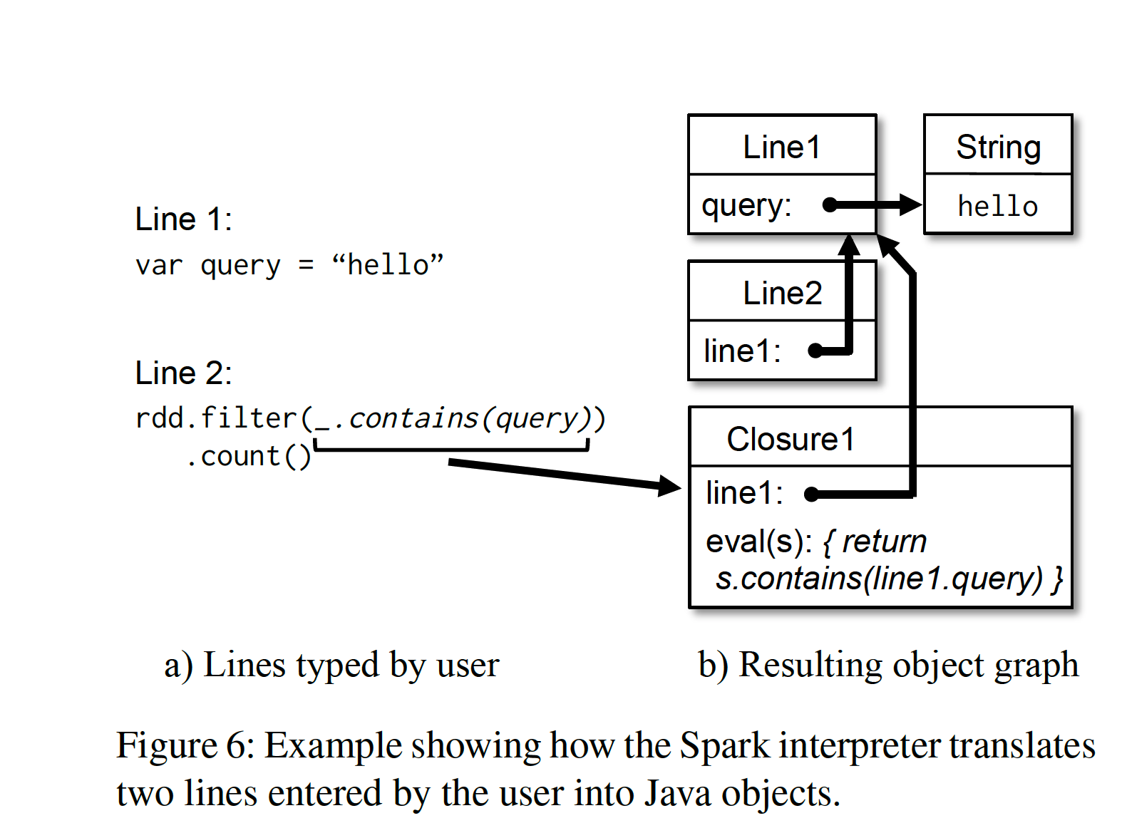spark interpreter

We found the interpreter very helpful for interactive queries on large datasets, and we plan to support more advanced query languages, such as SQL.

Memory Management

Spark provides three ways to store RDDs:

1. Unserialized Java objects in memory
2. Serialized data in memory
3. Disk

Since Spark runs on the JVM, the first storage method provides the fastest access, and the second allows users to sacrifice some performance for more efficient memory utilization. When data scales are too large to fit in memory, the third method is very useful.

To effectively utilize limited memory, we adopt an LRU-style eviction policy at the RDD partition level. That is, when we newly compute an RDD partition, if we find that memory is insufficient, we evict the least recently used RDD partition from memory. However, if this least recently used partition belongs to the same RDD as the newly computed partition, we continue searching until we find a partition that does not belong to the same RDD as the current partition and is the least recently used. Because most Spark computations are applied to entire RDDs, this prevents these partitions from being repeatedly computed and evicted. This policy worked well at the time the paper was written; however, we still provide users with interfaces for deep control — specifying storage priority.

Currently, each Spark instance has its own separate memory space; we plan to provide unified memory management across Spark instances in the future.

Checkpointing

Although all failed RDDs can be recomputed through lineage, for some RDDs with particularly long lineage, this would be a very time-consuming operation. Therefore, providing RDD-level external storage checkpointing may be very useful.

For RDDs with very long lineage graphs and many wide dependencies in the lineage graph, checkpointing to external storage is very helpful, because the loss of one or two partitions may trigger a full recomputation. For such long and complex computation topologies, recomputing based on the lineage graph would undoubtedly waste a lot of time. For RDDs with only narrow dependencies and not-so-long lineage graphs, checkpointing to external storage may be more costly than beneficial, because they can be easily computed in parallel.

Spark currently provides a checkpointing API (passing the REPLICATE flag to the persist function), and then leaves the decision of whether to persist it to the user. But we are considering whether some automatic checkpointing can be performed. Since the scheduler knows the memory footprint and computation time of each dataset, we may selectively persist certain key RDDs to minimize downtime recovery time.

Finally, due to the read-only nature of RDDs, we do not need to overly consider consistency issues when checkpointing as in general shared memory models. Therefore, background threads can silently perform these tasks without affecting the main workflow, and complex distributed snapshot algorithms need not be used to solve consistency issues.

Annotations

[1] Implicit vs. Explicit: Here, explicit means completely constructing the concept of a dataset, defining its connotation and boundaries, and making some extensions based on it. Implicit means de facto data reuse, but without defining the format of the reused data.

[2] Declarative vs. Imperative Languages: Examples of the former include SQL and HTML; the most common example of the latter is Shell, and other common programming languages such as C, Java, and Python also fall into this category. The advantage of the former is that it decouples “what to do” from “how to do it,” thereby enabling the development of different execution engines to optimize “how to do it” for different scenarios. The latter tells the machine to execute specific operations in a specific order, consistent with intuition, which is the approach of general programming languages.

---

我是青藤木鸟，一个喜欢摄影、专注大规模数据系统的程序员，欢迎关注我的公众号：“木鸟杂记”，有更多的分布式系统、存储和数据库相关的文章，欢迎关注。 关注公众号后，回复“资料”可以获取我总结一份分布式数据库学习资料。 回复“优惠券”可以获取我的大规模数据系统付费专栏《系统日知录》的八折优惠券。

我们还有相关的分布式系统和数据库的群，可以添加我的微信号：qtmuniao，我拉你入群。加我时记得备注：“分布式系统群”。 另外，如果你不想加群，还有一个分布式系统和数据库的论坛（点这里），欢迎来玩耍。