 over BLOB Storage Architecture
Overview
First, let me explain what BLOB means. Its full English name is Binary Large OBjects, which can be understood as large objects in arbitrary binary format; in Facebook’s context, these are images, videos, and documents uploaded by users. This data has the characteristics of created once, read many times, never modified, and occasionally deleted.
Previously, I briefly translated Facebook’s predecessor work — Haystack. As the business grew and data volume increased further, the old approach no longer worked. If all BLOBs were stored using Haystack, due to its triple-replication implementation, the cost-effectiveness at this scale would be very low. However, completely using network mounts + traditional disks + Unix-like (POSIX) file systems for cold storage couldn’t keep up with reads. Thus, the divide and conquer approach, most commonly used in computer science, came into play.
They first counted the relationship between BLOB access frequency and creation time, then proposed the concept of hot and cold distribution in BLOB access over time (similar to the long-tail effect). Based on this, they proposed a hot/warm separation strategy: using Haystack as hot storage to handle frequently accessed traffic, and using F4 to handle the remaining less frequently accessed BLOB traffic. Under this assumption (F4 only stores data that basically doesn’t change much and has relatively low access volume), F4’s design can be greatly simplified. Of course, there is a dedicated routing layer above both to shield the underlying details, make decisions, and route requests.
For Haystack, seven years had passed since its paper was published (07~14). Relative to that time, a few minor updates were made, such as removing the Flag bit, and adding a journal file in addition to the data file and index file, specifically to record deleted BLOB entries.
For F4, the main design goal is to minimize the effective replication factor (effective-replication-factor) as much as possible while ensuring fault tolerance, to address the growing demand for warm data storage. Furthermore, it is more modular and has better scalability, meaning it can smoothly scale by adding machines to cope with continuous data growth.
To summarize, the main highlights of this paper are hot/warm separation, erasure coding, and geo-replication.
Author: Muniao’s Notes https://www.qtmuniao.com, please indicate source when reprinting
Data Scale
By 2014, Facebook had over 400 billion images.
Access Frequency Heatmap
The paper concludes that an access frequency heatmap exists, creation time is a key factor affecting its changes, and warm data keeps growing.
The paper’s measurement method is also simple: tracking the access frequency curves of different types of BLOB data on their website as creation time changes. The access frequency of data less than one day old is about 100 times that of data one year old. I won’t list the specific data here; you can check it in the paper.
Then the paper explores a boundary for distinguishing hot data and warm data. Through analysis of how access frequency and deletion frequency change with creation time, for most BLOBs, an approximate value is obtained: one month. But there are two exceptions: one is user avatars, which are always hot data; the other is ordinary images, for which a three-month threshold is used.
Hot data is always the head data, growing relatively slowly. But historical data, that is, warm data, has an increasingly longer tail over time, which inevitably requires corresponding adjustments to the storage architecture.
Overall Storage System Architecture
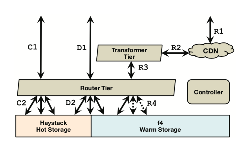
The design principle is to make each component as simple, cohesive, and highly aligned with the work it undertakes as possible. This is a principle emphasized since UNIX. The figure below shows the overall architecture, including creation (C1-C2, handled by Haystack), deletion (D1-D2, mostly handled by Haystack, with a small portion handled by f4), and reading (R1-R4, jointly handled by Haystack and f4).
over BLOB Storage Architecture
As described in the Haystack paper, we batch a group of BLOBs into a logical volume, minimizing meta information as much as possible to reduce the number of IO operations. Each logical volume is designed with a capacity of around 100GB. Before it is full, it is in an unlocked state; once capacity is reached, it becomes locked, only allowing reads and deletes.
Each volume contains three files: a data file, an index file, and a journal file. As mentioned in the Haystack paper, the data file records the BLOB itself and its metadata, and the index file is a snapshot of the in-memory lookup structure. The journal file is new; it performs deletion operations by recording all deleted BLOBs. In the original Haystack paper, deletion was implemented by directly modifying the index file and data file. In the unlocked phase, all three files can be read and written; in the locked phase, only the journal file can be read and written, while the other two files become read-only.
Controller
Oversees the entire system, such as provisioning new storage machines; maintaining a pool of unlocked volumes; ensuring all logical volumes have sufficient physical volume backups; creating physical volumes on demand; performing periodic maintenance tasks, such as compaction and garbage collection.
Routing Tier
The routing tier is responsible for providing the external interface for the BLOB storage system. It shields the underlying implementation of the system, making it easy to add subsystems like f4. All machines in the routing tier have the same role, because this layer stores all state (e.g., logical volume to physical volume mappings) in a separate database (collecting all related state for external storage makes the remaining parts stateless and smoothly scalable, which is also a commonly used principle in system design). This allows the routing tier to scale smoothly without depending on other modules.
For read requests, the routing module parses the logical volume id from the BLOB id, then finds all corresponding physical volume information based on the mapping read from the database. Generally, data is fetched from the nearest host; if that fails, a timeout event is generated, and the next physical volume’s host is tried.
For create requests, the routing module selects a logical volume with free space, then sends the BLOB to all corresponding physical volumes for writing (parallel, chained, or serial?). If any problem is encountered, the write is aborted, the already written data is discarded, and another available logical volume is selected to repeat the above process. (Looks like parallel writes, and the fault tolerance strategy is also super crude.)
For delete requests, the routing module sends them to all corresponding physical volumes (and then quickly returns), and the corresponding physical host programs asynchronously perform the deletion, retrying on errors until all corresponding BLOBs on all physical volumes are successfully deleted. (Simple, but I don’t know whether the implementation writes to the journal file before returning, or just marks it in memory. The corresponding BLOB in the data file is definitely only deleted during compaction.)
By hiding implementation details, the routing tier enables the transparent construction of warm storage. When a volume is moved from hot storage to warm storage, it exists on both for a period of time. After the effective (logical volume to physical volume) mapping is updated, client requests will be transparently directed to warm storage.
Transformer Tier
The transformer tier is responsible for handling transformation operations on retrieved BLOB data, such as image scaling and cropping. In Facebook’s older system versions, these compute-intensive operations were completed on the storage nodes.
Adding a transformer tier can free storage nodes to focus on providing storage services. Separating compute tasks also benefits independently scaling the storage tier and transformer tier. Furthermore, it allows us to precisely control storage node capacity to exactly meet demand. Going further, it enables us to make better hardware selections for different task types. For example, we can design storage nodes with large numbers of hard drives but only one CPU and a small amount of memory.
Caching Stack
Initially designed to handle hotspot BLOB data requests, relieving pressure on the backend storage system. For warm storage, it can also reduce request pressure. Here, it refers to CDNs and caches provided by content delivery providers like Akamai.
Haystack Hot Storage
Haystack was originally designed to maximize IOPS as much as possible. By taking on all create requests, most delete requests, and high-frequency read requests, the design of warm storage can be greatly simplified.
As mentioned in the related paper, Haystack greatly improves IOPS by merging BLOBs and simplifying metadata. Specifically, this includes designing logical volumes as single files that collect a batch of BLOBs, using three physical volumes for redundant backup of the same logical volume, and so on.
After a read request arrives, the requested BLOB’s metadata is obtained in memory, and it is checked whether it has been deleted. Then, through physical file location + offset + size, the corresponding BLOB data is obtained with only one IO.
When a host receives a create request, it synchronously appends BLOB data to the data file, then updates in-memory metadata and writes changes to the index file and journal file (doesn’t the journal file only record delete operations?).
When a host receives a delete request, it updates the index file and journal file. But the corresponding data still exists in the data file; periodically we perform compaction to truly delete the data and reclaim the corresponding space.
Fault Tolerance
Haystack achieves fault tolerance for disks, hosts, racks, and even datacenters through a triple-replica strategy: placing one replica on different racks in the same datacenter, and another replica in a different datacenter. Then RAID-6 (1.2x redundant data encoding, capable of correcting small-range errors, you can read articles on error correction codes) provides additional disk fault tolerance, adding another layer of insurance. But the cost is an effective replication factor of 3 * 1.2 = 3.6, which is Haystack’s limitation. Although it maximizes IOPS, it is not efficient in storage usage, causing a lot of BLOB data redundancy.
Expiry-Driven Content
Some types of BLOBs have a certain expiration time. For example, user-uploaded videos are converted from their original format to our storage format. After this, the original video needs to be deleted. We avoid moving such expiry-driven data to F4, letting Haystack handle these frequent delete requests and reclaim space through frequent compaction.
f4 Design
The design goal is to be as efficient as possible on the basis of fault tolerance. That is, under the premise of tolerating disk errors, host failures, rack issues, and datacenter disasters, reduce the effective replication factor.
f4 Overview
f4 is a subsystem of the warm data storage architecture. It contains a series of data cells, each cell located in the same datacenter. Currently (2014), a cell contains 14 racks, each rack has 15 hosts, and each host has thirty 4TB hard drives. The cell is responsible for storing logical volumes. When each logical volume is actually stored, its data is redundantly encoded using Reed-Solomon code (RS coding, abbreviated as RS, an important member of the RAID-6 standard mentioned earlier). For example, RS(n, k) means for every n bits stored, k additional bits are encoded, tolerating up to k bit errors. This encoding method can solve disk, host, and rack errors.
Furthermore, XOR coding is used to solve cross-datacenter or geographic errors. We select an equal number of volumes/stripes/blocks from two different datacenters to pair, then store the XOR of each pair in a third datacenter.
Individual f4 Cell
Each f4 data cell only handles locked volumes, meaning it only supports read and delete operations. Data files and index files are read-only; the journal file in Haystack does not exist in f4. We use another method to achieve the effect of “deletion”: each BLOB is encrypted before storage, and the encryption key is stored in an external database. When responding to a delete request, only the key corresponding to the BLOB needs to be deleted (a bit clever, providing privacy guarantees for users and reducing delete operation latency to very low).
Because the index file is relatively small, it directly uses triple-replica storage to ensure reliability, saving the extra complexity brought by encoding and decoding. Data files are encoded using Reed-Solomon with n=10, k=4. Specifically, each data file is split into n consecutive data blocks, each with a fixed size b (if the last block is not full and cannot fit a new BLOB, pad with zeros at the end; similar padding is also a commonly used technique for data alignment); for every n such blocks, k parity blocks of the same size are generated, so n+k blocks form a logical stripe. Any two blocks on the same stripe are called companion blocks. During normal reads, data can be directly read from the data blocks (I guess those n blocks, without extra computation to restore, to be verified by Reed-Solomon principles and specific implementation). If some blocks are unavailable, any n blocks from the same stripe are taken, decoded, and restored; furthermore, there is a property that reading n corresponding segments from n blocks (e.g., a certain BLOB) can also be decoded (both properties are determined by the encoding, similar to a system of n-variable linear equations with k redundant equations).
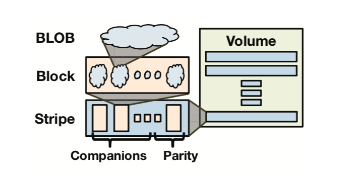 BLOBs in Block in Stripes in Volumes
Usually b is 1GB, meaning each data block is 1GB (there’s a question here: it looks like each Block is still inside the Volume, not separately extracted, so locating a physical block requires the volume file handle + offset + length). Choosing this size has two considerations: one is to minimize the probability of BLOBs spanning blocks, reducing the frequency of multiple IOs needed to read a BLOB; the other is to reduce the total amount of metadata that blocks need to maintain. The reason for not choosing a larger size is that reconstruction would be more costly (but why exactly 1GB?).
Below is the architecture diagram, next we introduce each module one by one.
overall architecture
Name Node
The name node maintains the mapping of data blocks and parity blocks to the storage nodes that actually store these blocks (i.e., the storage nodes in the next section); these mappings (using standard techniques? or referencing GFS, didn’t quite understand, leaving a pit to fill after reading GFS) are assigned to storage nodes. The name node uses primary-backup strategy for fault tolerance.
Storage Nodes
Storage nodes are the main component of a cell, handling all regular read and delete requests. They expose two APIs: the Index API is responsible for providing volume existence checks and location information; the File API provides actual data access. (The difference between File API and Data API probably lies in that the former provides an upper-level abstract BLOB operation interface, while the latter exposes underlying data block access interface.)
Storage nodes store the index file (including BLOB to volume mapping, offset, and length) on disk and load it into a custom in-memory storage structure. They also maintain the mapping from volume offset to physical data block (since a volume is cleanly cut into many blocks, locating the logical position of a data block requires recording its volume + offset). Both pieces of information are stored in memory to avoid disk IO (it seems there were also changes later, as SSDs became cheaper, storing on SSD is also possible).
Because each BLOB is encrypted, its key is stored in external storage, usually a database. Deleting its key achieves de facto BLOB deletion, thus avoiding data compaction (why not reclaim that deleted space? After all, for warm storage, deletions are only a small part, and the previous warm storage assumption is used here); it also saves using a journal file to track deletion information.
Below describes the read flow. First, use the Index API to check whether the file exists (R1 process), then forward the request to the storage node where the BLOB’s data block resides. The Data API provides access to data blocks and parity blocks. Under normal circumstances, read requests are directed to the appropriate storage node (R2 process), and then the BLOB is directly read from its block (R3). In failure cases, all intact n blocks from the n+k companion blocks are read through the Data API and sent to the backoff node for reconstruction.
During actual data read (whether the normal R1-R3 flow or the error fallback R1, R4, R5 flow), the routing tier reads the BLOB’s corresponding key from the external database in parallel, then performs decryption at the routing tier. This is a compute-intensive task; placing it here lets the data layer focus on storage, and both layers can be independently scaled.
Backoff Nodes
Responsible for providing a fallback solution when the normal read flow encounters errors.
When failures occur in a cell, some blocks become unavailable and need to be recovered online from companion blocks and parity blocks. Backoff modules are IO-sparse and compute-intensive nodes, handling these compute-intensive online recovery operations.
Backoff modules expose the File API to handle fallback retries when normal reads fail (R4). At this point, the read request has already been parsed by a primary volume-server into a tuple of data file, offset, and length. The backoff node reads the corresponding offset and length information from the n-1 companion blocks and k parity blocks, excluding the damaged data block. Once n responses are received (probably sent in parallel? Then to save time, start working upon receiving any n responses for error correction?).
Of course, to care for read latency, each online fallback read correction only recovers the data of the corresponding BLOB rather than the information of the entire data block. Recovery of the entire data block is left to the rebuilder nodes to do offline.
Rebuilder Nodes
With a certain scale of civilian physical machines, disk and node failures are inevitable. Data blocks stored on damaged modules need to be rebuilt. Rebuilder nodes are storage-sparse and compute-intensive, responsible for silently performing rebuild work in the background. Each rebuilder node detects data block errors through probes (periodically scanning the range it is responsible for? or installing probes on each data node?) and reports them to coordinator nodes. Then, by taking n intact blocks from the companion blocks and parity blocks on the same stripe, it rebuilds the damaged node (if n+k has other broken modules, they are probably rebuilt together). This is a very heavy processing procedure and brings enormous network and IO load to storage nodes. Therefore, rebuilder nodes throttle their throughput to prevent adverse effects on normal user requests. Coordinating and scheduling rebuild work to minimize data loss risk is the job of coordinator nodes.
Coordinator Nodes
A data cell needs many daily ops tasks, such as scheduling (roughly determining a rebuild order and distributing among different rebuilder nodes) damaged data block rebuilds, adjusting current data distribution to minimize data unavailability probability. Coordinator nodes are also storage-sparse and compute-intensive, used to execute cell-scoped tasks.
As mentioned earlier, different blocks on a data stripe need to be dispersed in different data fault tolerance zones to maximize reliability. However, after failures, rebuilds, and replacements, there will inevitably be some non-compliant situations, such as two blocks from the same stripe being placed in the same data fault tolerance zone. Coordinator nodes run a balancing placement process to check data block distribution in a cell. Like rebuild operations, this also brings considerable extra disk and network load to storage nodes, so coordinator nodes also self-throttle to reduce impact on normal requests.
Geo-Replication
A single f4 data cell exists in one datacenter, making it difficult to withstand datacenter failures. Therefore, initially, we placed two identical data cells in different datacenters, so that if one fails, the other can still respond to requests. This reduces the effective replication factor from Haystack’s 3.6 to 2.8.
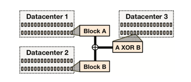 geo replicated xor coding
Considering that datacenter-level failures are still rare, we found a way to further reduce the effective replication factor — of course, it also reduces throughput. However, the current XOR scheme can further achieve an effective replication factor of 2.1.
The geo-replicated XOR coding scheme provides datacenter-level fault tolerance by XORing two different volumes (same size) and storing the result in a third datacenter. As shown in Figure 9, each data volume’s data blocks and parity blocks are XORed with an equal quantity of other data blocks or parity blocks (called buddy blocks) to obtain XOR blocks. The indices of these XOR blocks are also simply stored in triple replicas.
Once a datacenter problem causes an entire volume to be unavailable, read requests are routed to a geo-bakoff node, then corresponding BLOB data is fetched from the two buddy nodes and XOR node datacenters to reconstruct the damaged BLOB. XOR coding was chosen because it is simple and meets the needs.
Load factor calculation: (1.4 * 3) / 2 = 2.1
Summary
The basic ideas are roughly these; I won’t translate the rest. But the paper is a bit verbose, repeating the same point in different places several times, while one module is sometimes scattered across different sections, making it hard to form a whole picture. Here, I briefly summarize.
One data cell exists in one datacenter, containing 14 racks. One logical Volume, about 100GB, is divided into 100 1GB blocks; then every 10 blocks as a group (Companion Block) undergo data redundancy encoding (RS coding), producing 4 new parity blocks. These 14 data + parity blocks are called a stripe, placed on different racks for fault tolerance. The mapping of which blocks belong to which group is maintained in the Name Node.
On storage nodes, memory needs to maintain two mappings as index information: one is the mapping from BLOB id to volume, offset, and size; the other is the mapping from volume offset to the actual physical position of the Block. When a read request fails, the read request along with some metadata (such as the data block id and its offset on it) is directed to the Backoff Node. The backoff node gets the stripe’s other block position information from the Name Node based on the BLOB id’s Block id, and the offset, and only decodes all companion data for that BLOB, restores the BLOB, and returns it.
Furthermore, Coordinator Nodes obtain global data distribution and status information from probe heartbeats. Based on this, the coordinator assigns damaged modules to Rebuilder Nodes for data reconstruction; and balances and maintains all blocks on the stripe to be placed in different data fault tolerance zones.
Finally, after pairing all data blocks in two different datacenters, perform an XOR operation to obtain an XOR result, stored in a third datacenter. Thus, if any datacenter’s data stripe is damaged beyond what RS codes can save (for example, more than four racks fail), the other two datacenters’ data can be used for XOR operations to recover it.
Translation Glossary
data file: A file storing a bunch of BLOBs and their metadata
index file: A file recording BLOB offsets, lengths, and simple information in the data file, used to quickly seek and retrieve BLOBs.
journal file: In Haystack, used to record all delete requests.
effective-replica-factor: The ratio between actual occupied physical space and the logical data size to be stored.
companion block: The name for those n blocks among the n+k data blocks used for encoding.
parity block: The name for those k blocks among the n+k data blocks used for encoding.
warm storage: Relative to hot storage, refers to storage specifically built for data with not very high access frequency.
storage nodes, storage machines: Both refer to physical machines responsible for storing final data.
compact: In Haystack, the data file is periodically checked, copied once, but skipping all duplicate and already marked-deleted data, thereby reclaiming the corresponding space.
replica: A redundancy strategy. Errors are inevitable on cheap general-purpose machines; to have a fallback for recovery, the most common strategy is to store several extra copies. These identical data copies are called multiple replicas or multiple backups.
encryption key: The key used to encrypt BLOBs.
backoff node: Actually, I think translating it as a “fallback module” is also quite good, haha — it handles errors by taking n companion blocks to recover.
cell: A unit of data deployment and rollback consisting of 14 racks, with 15 machines on each rack.
volume: Divided into logical volumes and physical volumes, containing multiple data stripes.
stripe: A collection of original n data blocks and generated k parity blocks.
block: Generally about 1GB, dispersed in different fault tolerance units.