After Spark, UC Berkeley Launches a New Generation AI Compute Engine — Ray

Introduction

Following Spark, the UC Berkeley AMP Lab has launched another heavyweight high-performance AI compute engine — Ray, claiming to support millions of task schedules per second. How does it achieve this? After trying it out, here is a brief summary:

1. Minimalist Python API: By adding the ray.remote decorator to function or class definitions and making some minor changes, single-machine code can be turned into distributed code. This means not only can pure functions be executed remotely, but a class can also be registered remotely (Actor model), maintaining a large amount of context (member variables) within it, and remotely calling its member methods to change that context.
2. Efficient Data Storage and Transmission: On each node, a local object store is maintained through shared memory (multi-process access without copying), and data exchange between different nodes is performed using the specially optimized Apache Arrow format.
3. Dynamic Graph Computation Model: Thanks to the first two points, the future handles returned by remote calls are passed to other remote functions or actor methods. That is, complex computation topologies are built through nested remote function calls, and dynamic triggered execution is based on the publish-subscribe model of the object store.
4. Global State Maintenance: The global control state (rather than data) is maintained using Redis shards, allowing other components to easily scale smoothly and recover from failures. Of course, each Redis shard avoids single points of failure through chain-replica.
5. Two-level Scheduling Architecture: Divided into local scheduler and global scheduler; task requests are first submitted to the local scheduler, which tries to execute tasks locally to reduce network overhead. When resource constraints, data dependencies, or load conditions do not meet expectations, they are forwarded to the global scheduler for global scheduling.

Of course, there are still areas for optimization, such as Job-level encapsulation (for multi-tenant resource allocation), the garbage collection algorithm to be optimized (for the object store, currently just a crude LRU), multi-language support (Java was recently supported, but it is unclear how well it works), etc. However, its flaws do not hide its merits; its architectural design and implementation ideas still have many aspects worth learning from.

Author: Muniao’s Notes https://www.qtmuniao.com, please indicate the source when reposting

Motivation and Requirements

(The motivation for developing Ray started with reinforcement learning (RL), but due to the powerful expressiveness of its computation model, its use is by no means limited to RL. This section uses the description of RL system requirements as an opportunity to introduce Ray’s initial design direction. However, since I am not very familiar with reinforcement learning, some terms may be inaccurately expressed or translated. If you are only interested in its architecture, you can skip this section entirely.)

RL system example

Figure 1: An example of an RL system

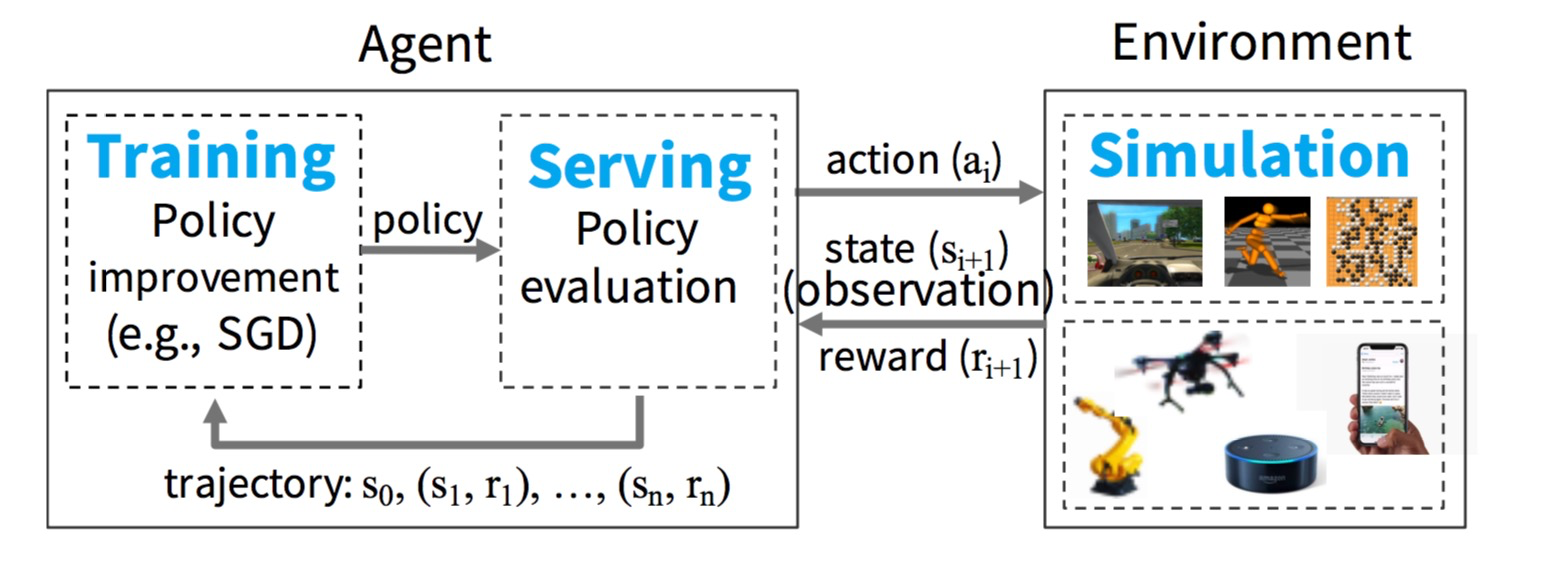
We start by considering the basic components of an RL system and gradually refine Ray’s requirements. As shown in Figure 1, in the setting of an RL system, an agent repeatedly interacts with an environment. The agent’s goal is to learn a policy that maximizes reward. A policy is essentially a mapping from states in the environment to actions. As for the environment, agent, state, action, and reward value definitions, these are determined by the specific application.

To learn a policy, the agent typically performs two steps: 1) policy evaluation and 2) policy improvement. To evaluate a policy, the agent continuously interacts with the environment (usually a simulated environment) to produce trajectories. A trajectory is a sequence of pairs (state, reward value) generated under the current environment and given policy. Then, the agent uses these trajectories to feedback and optimize the policy, that is, updating the policy in the gradient direction of maximizing the reward value. Figure 2 shows pseudocode for an example of how an agent learns a policy. This pseudocode evaluates the policy by calling rollout(environment, policy), thereby generating simulated trajectories. train_policy() then uses these trajectories as input, calling policy.update(trajectories) to optimize the current policy. This process is repeated iteratively until the policy converges.

// evaluate policy by interacting with env. (e.g., simulator) 
rollout(policy, environment):
    trajectory = []
    state = environment.initial_state()
    while (not environment.has_terminated()):
        action = policy.compute(state) // Serving
        state, reward = environment.step(action) // Simulation 
        trajectory.append(state, reward)
    return trajectory
    
// improve policy iteratively until it converges 
train_policy(environment):
    policy = initial_policy()
    while (policy has not converged):
        trajectories = [] 
        for i from 1 to k:
            // evaluate policy by generating k rollouts 
            trajectories.append(rollout(policy, environment)) 
            // improve policy
            policy = policy.update(trajectories) // Training 
    return policy

Figure 2: Typical pseudocode for learning a policy

From this perspective, a computation framework for RL applications needs to efficiently support model training (training), online prediction (serving), and platform simulation (simulation) (as shown in Figure 1). Next, we briefly explain these workloads.

Model training generally involves running stochastic gradient descent (SGD) models in a distributed environment to update the policy. Distributed SGD usually relies on allreduce aggregation steps or a parameter server.

Online prediction uses a trained policy to make action decisions based on the current environment. Prediction systems typically require reduced prediction latency and increased decision frequency. To support scaling, it is best to distribute the load across multiple nodes for collaborative prediction.

Finally, most existing RL applications use simulations to evaluate policies — because existing RL algorithms are not sufficient to efficiently sample from interactions with the physical world alone. These simulators span a wide range of complexity. Some may only take a few milliseconds (such as simulating moves in a chess game), while others may take several minutes (such as simulating a realistic environment for an autonomous driving vehicle).

Compared with supervised learning, where model training and online prediction can be handled in different systems, in RL all three workloads are tightly coupled in a single application, and the latency requirements between different workloads are very strict. None of the existing systems can support all three workloads simultaneously. In theory, multiple dedicated systems could be combined to provide all capabilities, but in practice, the latency of result transfer between subsystems is intolerable in RL. Therefore, RL researchers and practitioners have had to build multiple one-off dedicated systems for each requirement separately.

These current situations require the development of a brand-new distributed framework for RL that can effectively support training, prediction, and simulation. In particular, such a framework should have the following capabilities:

Support fine-grained, heterogeneous computation. RL computations often run for durations ranging from a few milliseconds (performing a simple action) to several hours (training a complex policy). In addition, model training usually requires various heterogeneous hardware support (such as CPU, GPU, or TPU).

Provide a flexible computation model. RL applications have both stateful and stateless types of computation. Stateless computation can be executed on any node in the system, thereby facilitating load balancing and on-demand data transfer. Therefore, stateless computation is very suitable for fine-grained simulation and data processing, such as extracting features from video or images. In contrast, stateful computation is suitable for implementing parameter servers, performing repeated iterations on data supporting GPU computation, or running third-party simulators that do not expose internal state parameters.

Dynamic execution capability. Many modules in RL applications require dynamic execution because the order in which their computations complete is not always predetermined (for example, the completion order of simulations), and the result of one computation can determine whether several future computations are executed (for example, the result of a simulation will determine whether we run more simulations).

In addition, we propose two additional requirements. First, to efficiently utilize large clusters, the framework must support millions of task schedules per second. Second, the framework is not meant to support implementing deep neural networks or complex simulators from scratch, but must seamlessly integrate with existing simulators (such as OpenAI gym) and deep learning frameworks (such as TensorFlow, MXNet, Caffe, PyTorch).

Language and Computation Model

Ray implements a dynamic task graph computation model, that is, Ray models an application as a task graph that dynamically generates dependencies during execution. On top of this model, Ray provides the actor model and the task-parallel programming paradigm. Ray’s support for mixed computation paradigms distinguishes it from systems like CIEL, which only provides parallel task abstractions, and Orleans or Akka, which only provide actor model abstractions.

Programming Model

Task Model. A task represents a remote function executed on a stateless worker process. When a remote function is called, a future representing the task result is immediately returned (that is, all remote function calls are asynchronous, returning a task handle immediately after the call). Futures can be passed to ray.get() to obtain results in a blocking manner, or futures can be passed as arguments to other remote functions for non-blocking, event-triggered execution (the latter is the essence of constructing dynamic topology graphs). These two features of futures allow users to specify dependencies while constructing parallel tasks. The following table lists all of Ray’s APIs (quite concise and powerful, but there are many pitfalls in implementation, since all functions or classes decorated with ray.remote and their contexts must be serialized and sent to remote nodes, using the same cloudpickle as PySpark).

Name	Description
futures = f.remote(args)	Execute function f remotely. f.remote() can take objects or futures as inputs and returns one or more futures. This is non-blocking.
objects = ray.get(futures)	Return the values associated with one or more futures. This is blocking.
ready futures = ray.wait(futures, k, timeout)	Return the futures whose corresponding tasks have completed as soon as either k have completed or the timeout expires.
actor = Class.remote(args) futures = actor.method.remote(args)	Instantiate class Class as a remote actor, and return a handle to it. Call a method on the remote actor and return one or more futures. Both are non-blocking.

Table 1 Ray API

Remote functions act on immutable objects and should be stateless and side-effect free: the output of these functions depends only on their inputs (pure functions). This means idempotence (idempotence); if an error occurs while obtaining a result, the function only needs to be re-executed, thereby simplifying fault-tolerant design.

Actor Model (Actors). An actor object represents a stateful computation process. Each actor object exposes a set of member methods that can be called remotely and executed sequentially in the order they are called (that is, within the same actor object, execution is serial to ensure the actor state is correctly updated). The execution process of an actor method is the same as a normal task; it is also executed remotely (each actor object corresponds to a remote process) and immediately returns a future; but unlike tasks, actor methods run on a stateful worker process. An actor object’s handle can be passed to other actor objects or remote tasks, allowing them to call these member functions on the actor object.

Tasks	Actors
Fine-grained load balancing	Coarse-grained load balancing
Support object locality (object store cache)	Poor locality support
High overhead for small updates	Low overhead for small updates
Efficient error handling	Higher overhead due to checkpoint recovery

Table 2 Task Model vs. Actor Model

Table 2 compares the task model and the actor model across different dimensions. The task model achieves fine-grained load balancing using cluster node load information and dependency data location information, that is, each task can be scheduled to an idle node that stores its required parameter objects; and it does not require much additional overhead because there is no need to set checkpoints and recover intermediate states. In contrast, the actor model provides extremely efficient fine-grained update support because these updates act on internal state (i.e., context information maintained by actor member variables) rather than external objects (such as remote objects, which need to be synchronized to local first). The latter usually requires serialization and deserialization (as well as network transmission, which is often time-consuming). For example, the actor model can be used to implement parameter servers (parameter servers) and GPU-based iterative computations (such as training). In addition, the actor model can be used to wrap third-party simulators or other objects that are difficult to serialize (such as certain models).

To satisfy heterogeneity and scalability, we have enhanced the API design in three aspects. First, to handle concurrent tasks of varying lengths, we introduced ray.wait(), which can return as soon as the first k results are satisfied; unlike ray.get(), which must wait until all results are satisfied before returning. Second, to handle tasks with different resource dimension (resource-heterogeneous) requirements, we allow users to specify the required resource amount (for example, decorator: ray.remote(gpu_nums=1)), so that the scheduling system can manage resources efficiently (providing a means of interaction so that the scheduling system is relatively less blind when scheduling tasks). Finally, for flexibility, we allow the construction of nested remote functions, meaning one remote function can call another remote function within it. This is crucial for achieving high scalability because it allows multiple processes to call each other in a distributed manner (this is very powerful; through proper function design, all parallelizable parts can be turned into remote functions, thereby improving parallelism).

Computation Model

Ray adopts a dynamic graph computation model, in which remote functions and actor methods are automatically triggered for execution when inputs are available (i.e., all input objects that the task depends on have been synchronized to the node where the task is located). In this section, we describe in detail how to build a computation graph (Figure 4) from a user program (Figure 3). This program uses the APIs in Table 1 to implement the pseudocode in Figure 2.

@ray.remote
def create_policy():
# Initialize the policy randomly. return policy

@ray.remote(num_gpus=1)
class Simulator(object):
  def __init__(self):
  # Initialize the environment. self.env = Environment()
    def rollout(self, policy, num_steps):
      observations = []
      observation = self.env.current_state()
      for _ in range(num_steps):
        action = policy(observation)
        observation = self.env.step(action)
        observations.append(observation)
      return observations

@ray.remote(num_gpus=2)
def update_policy(policy, *rollouts):
  # Update the policy.
  return policy

@ray.remote
def train_policy():
  # Create a policy.
  policy_id = create_policy.remote()
  # Create 10 actors.
  simulators = [Simulator.remote() for _ in range(10)] # Do 100 steps of training.
  for _ in range(100):
      # Perform one rollout on each actor.
      rollout_ids = [s.rollout.remote(policy_id)
                     for s in simulators]
      # Update the policy with the rollouts.
      policy_id =
          update_policy.remote(policy_id, *rollout_ids)
   return ray.get(policy_id)

Figure 3: Code implementing the logic of Figure 2 in Ray. Note that the @ray.remote decorator declares the annotated method or class as a remote function or actor object. After calling a remote function or actor method, a future handle is immediately returned, which can be passed to subsequent remote functions or actor methods to express data dependencies. Each actor object contains an environment object self.env, whose state is shared by all actor methods.

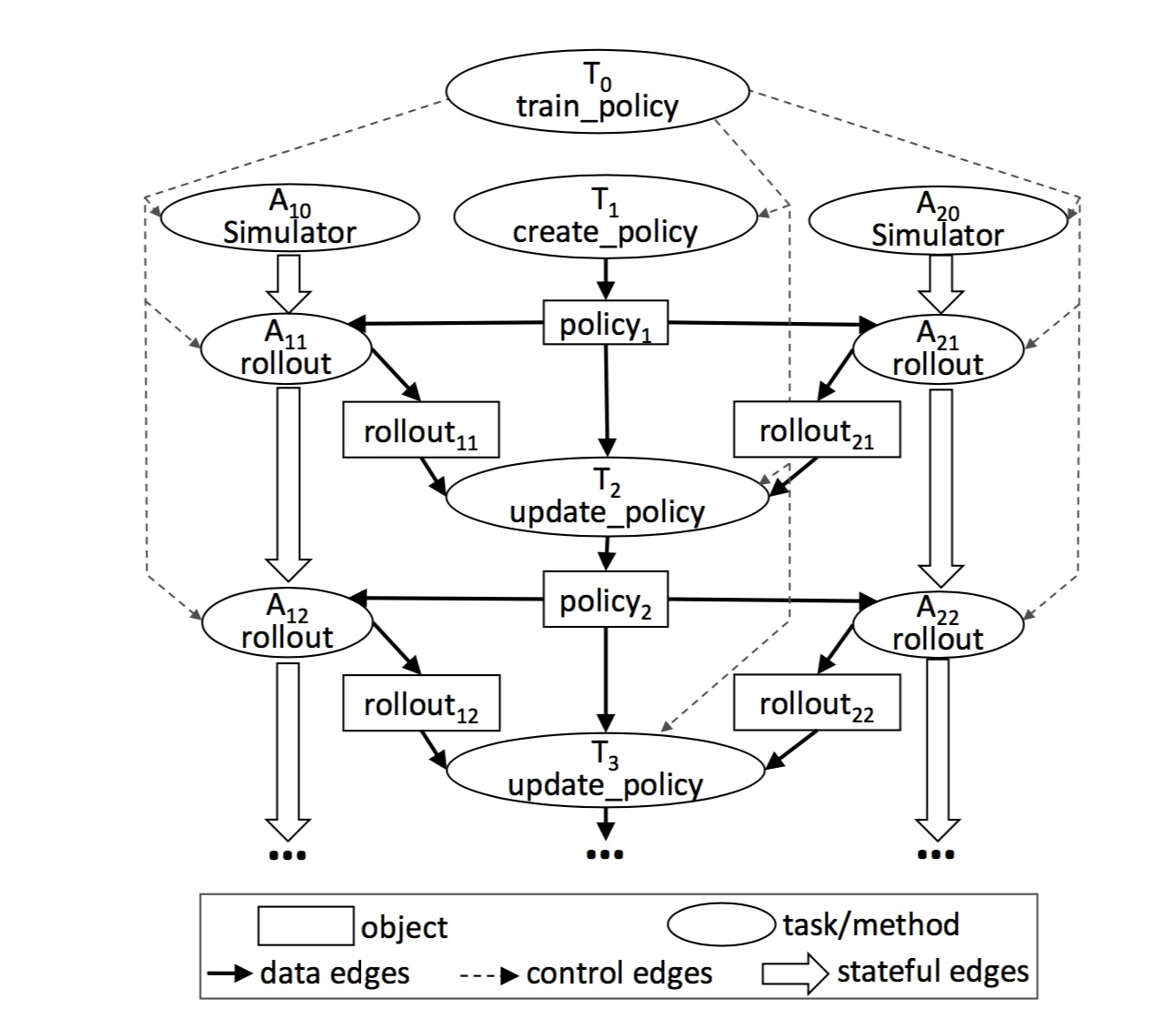
Without considering actor objects, there are two types of nodes in a computation graph: data objects and remote function calls (or tasks). Similarly, there are two types of edges: data edges and control edges. Data edges express dependency relationships between data objects and tasks. More precisely, if data object D is the output of task T, we add an edge from T to D. Similarly, if D is the input of task T, we add an edge from D to T. Control edges express computation dependencies caused by nested remote function calls, that is, if task T1 calls task T2, we add a control edge from T1 to T2.

In the computation graph, actor method calls are also represented as nodes. Except for one key difference, their dependency relationships with task calls are basically the same. To express the state dependency relationship formed by consecutive method calls on the same actor object, we add a third type of edge to the computation graph: on the same actor object, if actor method Mj is called immediately after Mi, we add a state edge from Mi to Mj (that is, after Mi is called, certain states in the actor object are changed, or member variables; then these changed member variables serve as implicit inputs for the Mj call; thus, an implicit dependency relationship is formed between Mi and Mj). In this way, all method calls acting on the same actor object will form a call chain (chain, see Figure 4) connected by state edges. This call chain expresses the sequential dependency relationship of method calls on the same actor object.

task graph

Figure 4: This graph corresponds to the train_policy.remote() call in Figure 3. Remote function calls and actor method calls correspond to tasks in the graph. The figure shows two actor objects A10 and A20; each actor object’s method calls (tasks marked as A1i and A2i) are connected by stateful edges, indicating that these calls share mutable actor state. There are control edges connecting from train_policy to the tasks it calls. To train multiple policies in parallel, we can call train_policy.remote() multiple times.

State edges allow us to embed actor objects into a stateless task graph because they express the implicit data dependency relationship between two actor method calls that share state and are sequential. The addition of state edges also allows us to maintain a lineage graph; like other dataflow systems, we track data lineage for reconstruction when necessary. By explicitly introducing state edges into the data lineage graph, we can conveniently reconstruct data, regardless of whether the data is produced by remote functions or actor methods (this will be discussed in detail in Section 4.2.3).

Architecture

Ray’s architecture consists of two parts:

1. The application layer that implements the API, currently including versions implemented in Python and Java.
2. The system layer that provides high scalability and fault tolerance, written in C++ and embedded in the package as CPython.

ray architecture

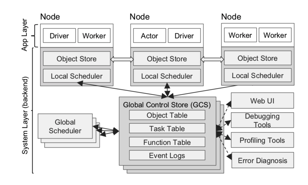
Figure 5: Ray’s architecture consists of two parts: the system layer and the application layer. The former implements the API and computation model; the latter implements task scheduling and data management to meet performance and fault tolerance requirements.

Application Layer

The application layer includes three types of processes:

• Driver: Used to execute user programs.
• Worker: A stateless process used to execute tasks assigned by the Driver or other Workers (remote functions, i.e., functions decorated with @ray.remote in user code). Workers are automatically started when nodes start, and generally the same number of Workers as CPUs are started on each physical machine (there are still some issues here: if the node is a container, it still gets the CPU count of the physical machine it resides on). When a remote function is declared, it is registered globally and pushed to all Workers. Each Worker executes tasks sequentially and does not maintain local state.
• Actor: A stateful process used to execute actor methods. Unlike Workers, which are started automatically, each Actor is explicitly started by a Worker or Driver on demand (i.e., when called). Like Workers, Actors also execute tasks sequentially; the difference is that the execution of the next task depends on the state generated or changed by the previous task (i.e., the member variables of the Actor).

System Layer

The system layer includes three main components: the Global Control Store (GCS), the distributed scheduler, and the distributed object store. All components can scale horizontally and support fault tolerance.

Global Control Store (GCS)

The global state store maintains global control state information for the system and is an original component of our system. Its core is a publish-subscribe key-value store. We use sharding to cope with scaling, and each shard uses chain replication (organizing all data replicas into a linked list to ensure strong consistency, see a 2004 paper) for fault tolerance. The motivation for proposing and designing such a GCS is to enable the system to perform millions of task creations and schedules per second, with low latency and convenient fault tolerance.

Fault tolerance for node failures requires a scheme that can record lineage information. Existing lineage-based solutions focus on coarse-grained parallelism (such as Spark’s RDD), so lineage information can be stored on a single node (such as Master or Driver) without affecting performance. However, this design is not suitable for fine-grained, dynamic workload types like simulation. Therefore, we decouple lineage information storage from other system modules so that it can scale independently and dynamically.

Maintaining low latency means minimizing task scheduling overhead as much as possible. Specifically, a scheduling process includes selecting a node, dispatching the task, pulling remote dependency objects, etc. Many existing information flow systems centrally store all object location, size, and other information on the scheduler, coupling the above scheduling processes together. When the scheduler is not a bottleneck, this is a very simple and natural design. However, considering the data volume and data granularity that Ray needs to handle, the central scheduler needs to be removed from the critical path (otherwise, if all scheduling goes through the global scheduler, it will definitely become a bottleneck). For primitives like allreduce, which are important for distributed training (frequent transmission, latency-sensitive), the overhead of going through the scheduler for each object transmission is intolerable. Therefore, we store object metadata in the GCS rather than the central scheduler, completely decoupling task dispatch from task scheduling.

Overall, the GCS greatly simplifies Ray’s overall design because it takes on all the state, thereby making all other parts of the system stateless. This not only simplifies fault tolerance support (i.e., each failed node only needs to read lineage information from the GCS when recovering), but also allows the distributed object store and scheduler to scale independently (because all components can obtain necessary information through the GCS). Another additional benefit is that it is more convenient to develop debugging, monitoring, and visualization tools.

Bottom-up Distributed Scheduler

As mentioned earlier, Ray needs to support millions of task schedules per second; these tasks may last only a few milliseconds. Most known scheduling strategies do not meet these requirements. Common cluster computing frameworks such as Spark, CIEL, and Dryad all implement a central scheduler. These schedulers have good locality characteristics but often have latencies of tens of milliseconds. Distributed schedulers like work stealing, Sparrow, and Canary can indeed achieve high concurrency, but they often do not consider data locality, or assume tasks belong to different jobs, or assume the computation topology is known in advance.

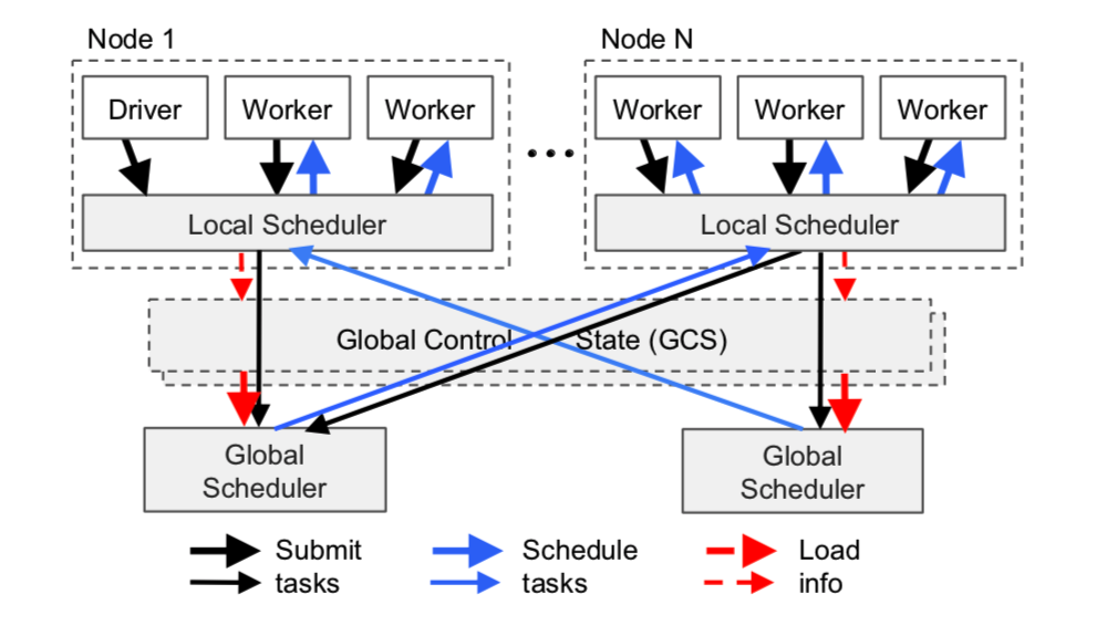
To meet the above requirements, we designed a two-level scheduling architecture, including a global scheduler and a local scheduler on each node. To avoid overloading the global scheduler, tasks created on each node are first submitted to the local scheduler. The local scheduler always tries to execute tasks locally unless its machine is overloaded (for example, the task queue exceeds a predefined threshold) or cannot satisfy the task’s resource requirements (for example, lacking a GPU). If the local scheduler finds that a task cannot be executed locally, it forwards it to the global scheduler. Since the scheduling system tends to schedule tasks locally first (i.e., at the leaf nodes of the scheduling structure hierarchy), we call it a bottom-up scheduling system (as can be seen, the local scheduler only schedules based on local load information of the node, while the global scheduler dispatches tasks based on global load; of course, the premise is that resource constraints must first be satisfied).

ray distributed scheduler

Figure 6 This is a schematic diagram of the scheduling system. Tasks are submitted bottom-up: tasks are first submitted by Drivers or Workers to the local scheduler, and then forwarded to the global scheduler for processing when needed. The thickness of the arrows in the figure represents the busyness of the requests.

The global scheduler determines scheduling strategy based on the load status of each node and resource request constraints. To elaborate, the global scheduler first determines all nodes that satisfy the task’s resource requirements, then selects the one with the smallest estimated waiting time, and schedules the task there. On a given node, the estimated waiting time is the sum of the following two times: 1) the task’s queuing time on the node (task queue length multiplied by average execution time); 2) the estimated transfer time for remote objects that the task depends on (size of all remote inputs divided by average bandwidth). The global scheduler obtains each node’s task queuing and available resource information through heartbeats, and gets the location and size of all task inputs from the GCS. Then, the global scheduler calculates the average task execution time and average transmission bandwidth using exponential moving average. If the global scheduler becomes a system bottleneck, we can instantiate more replicas to share the load; they share global state information through the GCS. In this way, our scheduling architecture has extremely high scalability.

Task Lifecycle

(Note: This part is translated from the design document in the code; note that this is only the design as of 2019.04.21)

During implementation, each task has the following states. At any point in time, a task will be in one of these states.

• Placeable: The task is ready to be scheduled to a (local or remote) node; how exactly it is scheduled was explained in the previous paragraph. Note that this state does not mean the placement location is finalized; it may be scheduled out from somewhere again.
• WaitActorCreation: An actor method (task) waits for its actor to be instantiated. Once the actor is created, the task is forwarded to the remote machine running the actor for processing.
• Waiting: Waiting for the task’s parameter requirements to be satisfied, that is, waiting for all remote parameter objects to be transferred to the local object store.
• Ready: The task is ready to be run, meaning all required parameters are already in the local object store.
• Running: The task has been dispatched and is running in the local worker process or actor process.
• Blocked: The current task is blocked because its dependent data is unavailable. For example, in a nested call, the task starts another remote task and waits for it to complete to obtain the result.
• Infeasible: The task’s resource requirements cannot be satisfied on any machine.

                                  ---------------------------------
                                 |                                 |
                                 |     forward                     | forward
                                 |----------------                 |
node with                  ------|                |   arguments    |
resources          forward|      |   resource     |     local      |   actor/worker
joins                     |      v  available     |    -------->   |    available
  ---------------------- Placeable ----------> Waiting           Ready ---------> Running
|                       | |  ^                    ^    <--------   ^               |   ^
|             |---------  |  |                    |    local arg   |               |   |
|             |           |  |                    |     evicted    |        worker |   | worker
|             |     actor |  |                    |                |       blocked |   | unblocked
|   resources |   created |  | actor              | ---------------                |   |
|  infeasible |           |  | created            | actor                          |   |
|             |           |  | (remote)           | created                        v   |
|             |           v  |                    | (local)                              Blocked
|             |     WaitForActorCreation----------
|             v
 ----Infeasible

In-Memory Distributed Object Store

To reduce task latency, we implemented an in-memory distributed storage system to store the inputs and outputs of each task (a stateless computation process). On each node, we implemented the object store using shared memory. This allows different tasks on the same node to share data with zero-copy overhead. As for the data format, we chose Apache Arrow.

If a task’s inputs (i.e., the function’s parameter objects) are not local, before the task is executed, the inputs are copied to the local object store. At the same time, after task execution, the outputs are also written to the local object store. Object copying eliminates potential bottlenecks caused by hot data and shortens execution time by restricting task data reads and writes to local memory. These practices increase the throughput of compute-intensive workloads, and many AI applications are compute-intensive. To reduce latency, we keep all used objects in memory, and only evict some objects from memory using the LRU algorithm when memory is insufficient (from the API, it can be seen that each node’s memory limit can be specified through parameters when starting the node. In addition, using LRU as a garbage collection algorithm is still a bit crude; if different types of task workloads run on the same Ray cluster, it may lead to resource contention, causing a large amount of resource swapping out and then reconstruction, thereby seriously affecting efficiency).

Like existing cluster computing frameworks (such as Spark, Dryad), the object store only accepts immutable data. This design avoids the need for complex consistency protocols (because object data never needs to be updated) and simplifies data fault tolerance support. When a node fails, Ray recovers any required objects by re-executing the object lineage graph (that is, it does not need to recover all states of the failed node, only the data required for subsequent computations needs to be recovered on demand; data that is not used can be lost). Before work begins, lineage information stored in the GCS tracks all stateless tasks and stateful actors; we use the former to reconstruct lost objects (combining with the previous paragraph, if a task has a large number of iterations and all are executed remotely, it will produce a large number of intermediate result objects, causing memory to burst, thereby squeezing out less frequently used but possibly later needed global variables, so LRU is a bit crude; I heard that a reference-counting-based GC is being considered).

To simplify implementation, our object store does not support distributed objects. That is, each object must fit in a single node’s memory and exist only on a single node. For large objects such as large matrices and tree structures, they can be split and processed at the application layer, for example, implemented as a collection.

Implementation

Ray is an active open-source project developed by UC Berkeley. Ray is deeply integrated with Python; you can install Ray via pip install ray. The entire code implementation includes approximately 40K lines, of which 72% is the system layer implemented in C++ and 28% is the application layer implemented in Python (as of now, support for Java has also been added). Each shard of the GCS uses a Redis key-val store and is only designed for single key-value pair operations. GCS tables are smoothly scaled by sharding according to task ID and data object collections. Each shard uses chained replication for fault tolerance. We implemented both the local scheduler and the global scheduler as single-threaded, event-driven processes. The local scheduler caches local object metadata, blocked task queues, and task queues waiting to be scheduled. To seamlessly transfer very large objects between object stores on different nodes, we slice large objects and use multiple TCP connections for parallel transmission.

Putting All the Pieces Together

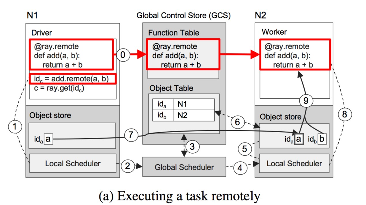
Figure 7 demonstrates Ray’s end-to-end workflow through a simple example of adding a and b (a and b can be scalars, vectors, or matrices) and returning c. The remote function add() is automatically registered in the GCS during initialization (ray.init) and then distributed to every worker process in the cluster. (Step 0 in Figure 7a)

Figure 7a shows each step of Ray’s operation when a driver process calls add.remote(a, b), and a and b are on nodes N1 and N2 respectively. The driver process submits the task add(a, b) to the local scheduler (step 1), and then the task request is forwarded to the global scheduler (step 2) (as mentioned earlier, if the local task queue does not exceed the set threshold, the task can also be executed locally). Then, the global scheduler begins to look up the locations of parameters a and b in the GCS for the add(a, b) request (step 3), and decides to schedule the task to node N2 (because N2 has one of the parameters, b) (step 4). After the local scheduler on node N2 receives the request (finding that the local scheduling policy conditions are met, such as satisfying resource constraints and the queue not exceeding the threshold, it will start executing the task locally), it checks whether all input parameters for task add(a, b) exist in the local object store (step 5). Since object a is not in the local object store, the worker process looks up the location of a in the GCS (step 6). At this point, it finds that a is stored in N1, so it synchronizes it to the local object store (step 7). Since all input parameter objects for task add() exist in the local store, the local scheduler executes add() in the local worker process (step 8), accessing the input parameters through shared storage (step 9).

ray execute example

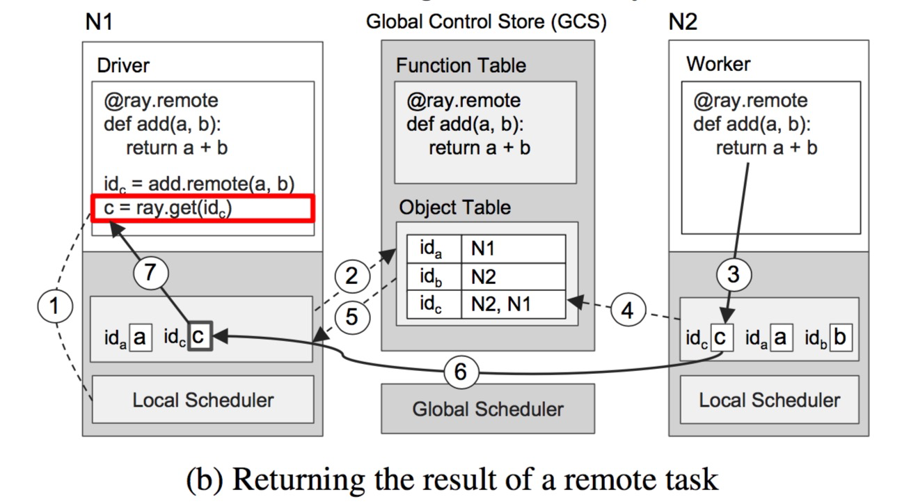
Figure 7b shows the step-by-step operations triggered by executing ray.get() on N1 and executing add() on N2. Once ray.get(id) is called, the user driver process on N1 checks whether the object c corresponding to this id (that is, the future value returned by the remote call add(). All object IDs are globally unique, which the GCS can guarantee) exists in the local object store (step 1). Since object c is not in the local object store, the driver process goes to the GCS to look up the location of c. At this point, it finds that c does not exist in the GCS, because c has not been created yet. So, the object store on N1 registers a callback function in the Object Table in the GCS to listen for the creation event of object c (step 2). Meanwhile, on node N2, the add() task completes execution, stores the result c in its local object store (step 3), and also adds the location information of c to the object store table in the GCS (step 4). The GCS detects the creation of c and triggers the callback function previously registered by the object store on N1 (step 5). Next, the object store on N1 synchronizes c from N2 (step 6), thus completing the task.

ray execute example b

Although this example involves a large number of RPC calls, in most cases the number of RPCs will be much smaller, because most tasks will be scheduled and executed locally, and the object information replied by the GCS will be cached by the local scheduler and global scheduler (but on the other hand, after executing a large number of remote tasks, the local object store is easily overwhelmed).

Terminology Cross-Reference

workloads: Workload, i.e., describing the work a task needs to do.

GCS: Global Control Store, global control information storage.

Object Table: An object table existing in the GCS, recording the location and other information of all objects (objectId -> location).

Object Store: Local object store, called Plasma in the implementation, i.e., the instance storing objects required by tasks.

Lineage: Bloodline information, pedigree information; i.e., the successive relationship graph of data transformations during computation.

Node: Node; each physical node in the Ray cluster.

Driver, Worker: Driver process and worker process; physically, both are processes on a Node. However, the former is generated when the user side uses ray.init and is destroyed when ray.shutdown is called. The latter is a stateless resident worker process started on each node when ray starts, generally the same number as the physical machine’s CPUs.

Actor: Actor object; at the language level, it is a class; at the physical level, it is manifested as an actor process on a certain node, maintaining all context within the actor object (actor member variables).

Actor method: Actor method; at the language level, it is a member method of a class; all its inputs include explicit function parameters and implicit member variables.

Remote function: Remote function, i.e., a function registered to the system via @ray.remote. When it is scheduled, it is called a Task.

Job, Task: The text uses the concepts of Job and Task a lot, but these two concepts are actually rather vaguely defined in CS, not as clear as processes and threads. In this paper, a Task is the encapsulation of a remote function (remote action) or an actor’s remote method (remote method). A Job does not currently exist in the implementation; it is only a logical concept, meaning the collection of all generated Tasks and produced states involved in running a piece of user-side code.

Scheduler: The paper uniformly uses scheduler, but sometimes refers to a part (local scheduler and global scheduler), which I translate as scheduler, and sometimes refers to the entirety of all schedulers in Ray, which I translate as scheduling system.

exponential averaging: I translated it as exponential moving average, although it does not say moving. For the past n items, a weighted average is performed with weights that increase exponentially over time. During calculation, it can be conveniently recursively calculated using the concept of a sliding window.

Future: This is not easy to translate; the general meaning is the return value handle in an asynchronous call. For more information, see Wikipedia Future and promise.

References

[1] Official documentation: https://ray.readthedocs.io/en/latest/

[2] System paper: https://www.usenix.org/system/files/osdi18-moritz.pdf

[3] System source code: https://github.com/ray-project/ray

---

我是青藤木鸟，一个喜欢摄影、专注大规模数据系统的程序员，欢迎关注我的公众号：“木鸟杂记”，有更多的分布式系统、存储和数据库相关的文章，欢迎关注。 关注公众号后，回复“资料”可以获取我总结一份分布式数据库学习资料。 回复“优惠券”可以获取我的大规模数据系统付费专栏《系统日知录》的八折优惠券。

我们还有相关的分布式系统和数据库的群，可以添加我的微信号：qtmuniao，我拉你入群。加我时记得备注：“分布式系统群”。 另外，如果你不想加群，还有一个分布式系统和数据库的论坛（点这里），欢迎来玩耍。