The originator of the “industrial assembly line,” the motor assembly of the Ford Model T, broke the assembly process into 29 steps, reducing assembly time from an average of twenty minutes to five minutes — a fourfold efficiency gain. The image below is sourced from.
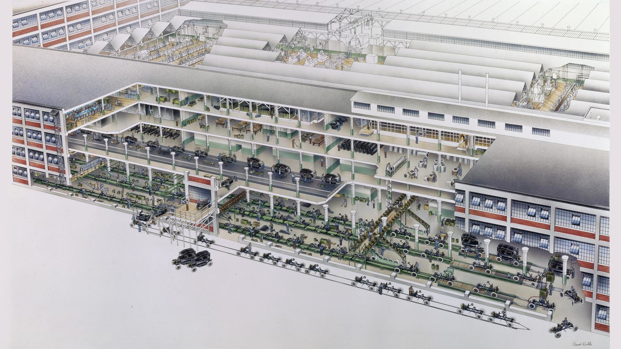 T-model-car.png
This assembly-line philosophy is ubiquitous in data processing. Its core concepts are:
- Standardized data collections: Corresponding to the object to be assembled, this is a consistent abstraction for the inputs and outputs of every stage in data processing. Consistency means that the output of any processing stage can serve as the input to any other processing stage.
- Composable data transformations: Corresponding to a single assembly step, this defines an atomic operation that transforms data. By combining various atomic operations, one can achieve powerful expressiveness.
Thus, the essence of data processing is: for different requirements, read and standardize the data collection, then apply different combinations of transformations.
Author: 木鸟杂记 https://www.qtmuniao.com/2023/08/21/unify-data-processing Please indicate the source when reprinting
Unix Pipes
Unix pipes are a truly great invention, embodying the consistent philosophy of Unix:
Programs should focus on one goal and do it as well as possible. Programs should be able to work together. Programs should handle text data streams, because that is a universal interface.
— Malcolm Douglas McIlroy, inventor of the Unix Pipe mechanism
The above three sentences perfectly embody the two points we mentioned: standardized data collections — text data streams from standard input and output; composable data transformations — programs that can work together (such as built-in Unix tools like sort, head, tail, and user-written programs that conform to pipe requirements).
Let’s look at an example of using Unix tools and pipes to solve a real-world problem. Suppose we have some log files about service access (var/log/nginx/access.log, example from DDIA Chapter 10), with each line of the log in the following format:
1 | // $remote_addr - $remote_user [$time_local] "$request" |
Our requirement is to find the five most popular pages in the log file. Using Unix Shell, we would write a command like this:
1 | cat /var/log/nginx/access.log | # read the file and output to stdout |
The above Shell command has the following characteristics:
- Each command implements a very simple function (high cohesion)
- All commands are composed through pipes (low coupling). Of course, this also requires that composable programs only read from standard input and write to standard output, with no other side effects (such as writing to files)
- Input and output are text-based rather than binary
In addition, another major advantage of Unix pipes is streaming data processing. That is, intermediate results are not all computed before being fed to the next command; instead, they are sent as they are computed, enabling multiple programs to execute in parallel — this is the essence of the pipeline.
Of course, pipes also have a drawback: they can only arrange linear pipelines, which limits their expressiveness.
GFS and MapReduce
MapReduce was proposed in Google’s 2004 paper MapReduce: Simplified Data Processing on Large Clusters as an algorithm for large-scale cluster parallel data processing. GFS is a disk-based distributed file system designed to be used in conjunction with MapReduce.
The MapReduce algorithm is mainly divided into three phases:
- Map: In parallel across different machines, execute a user-defined
map() → List<Key, Value>function on each data partition. - Shuffle: Re-partition the output of the map (KV pairs) by key, group them by key, and send them to different machines,
Key → List<Value>. - Reduce: In parallel across different machines, call the reduce function on the
List<Value>corresponding to each key output by the map.
(Image source: DDIA Chapter 10)
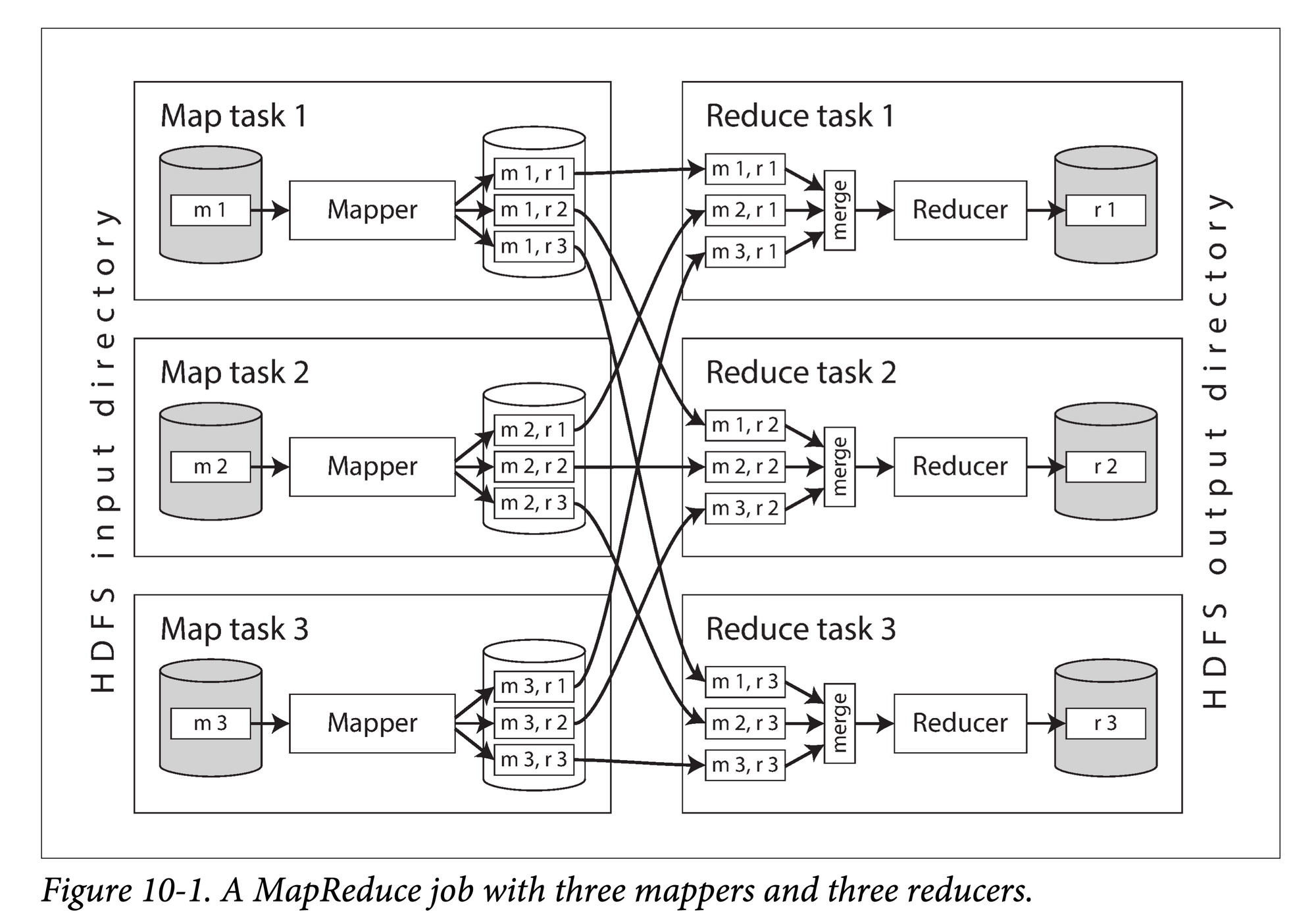 mapreduce.png
Each MapReduce program is a transformation of a dataset stored on GFS (a standardized dataset). In theory, we can meet arbitrarily complex data processing needs by combining multiple MapReduce programs (composable transformations).
But unlike pipes, the output of each MapReduce job must be materialized, i.e., fully written to the distributed file system GFS, before the next MapReduce job can execute. The benefit is that arbitrary, non-linear arrangements of MapReduce programs are possible. The downside is the very high cost, especially considering that files on GFS are multi-machine, multi-replica datasets, which means massive cross-machine data transfer and extra data copy overhead.
However, one must consider that groundbreaking innovations, however flawed at first, are gradually overcome through iteration. GFS + MapReduce is precisely such a pioneering system in the industry for processing massive data at the scale of large clusters.
Spark
Spark is an evolution designed to solve the problem that every intermediate dataset in MapReduce has to be written to disk.
First, Spark proposed a standard dataset abstraction — RDD, a memory-based dataset distributed across multiple machines in the form of partitions. Being memory-based means that intermediate results do not need to be written to disk, resulting in lower processing latency. Being partitioned means that when a machine fails, only a small number of partitions need to be recovered, rather than the entire dataset. Logically, we can treat it as a whole for transformation; physically, we use the memory of multiple machines to hold each partition.
Second, based on RDDs, Spark provides a rich set of flexibly composable operators, which is equivalent to “componentizing” some commonly used transformation logic, allowing users to use them out of the box. (Image source: RDD paper)
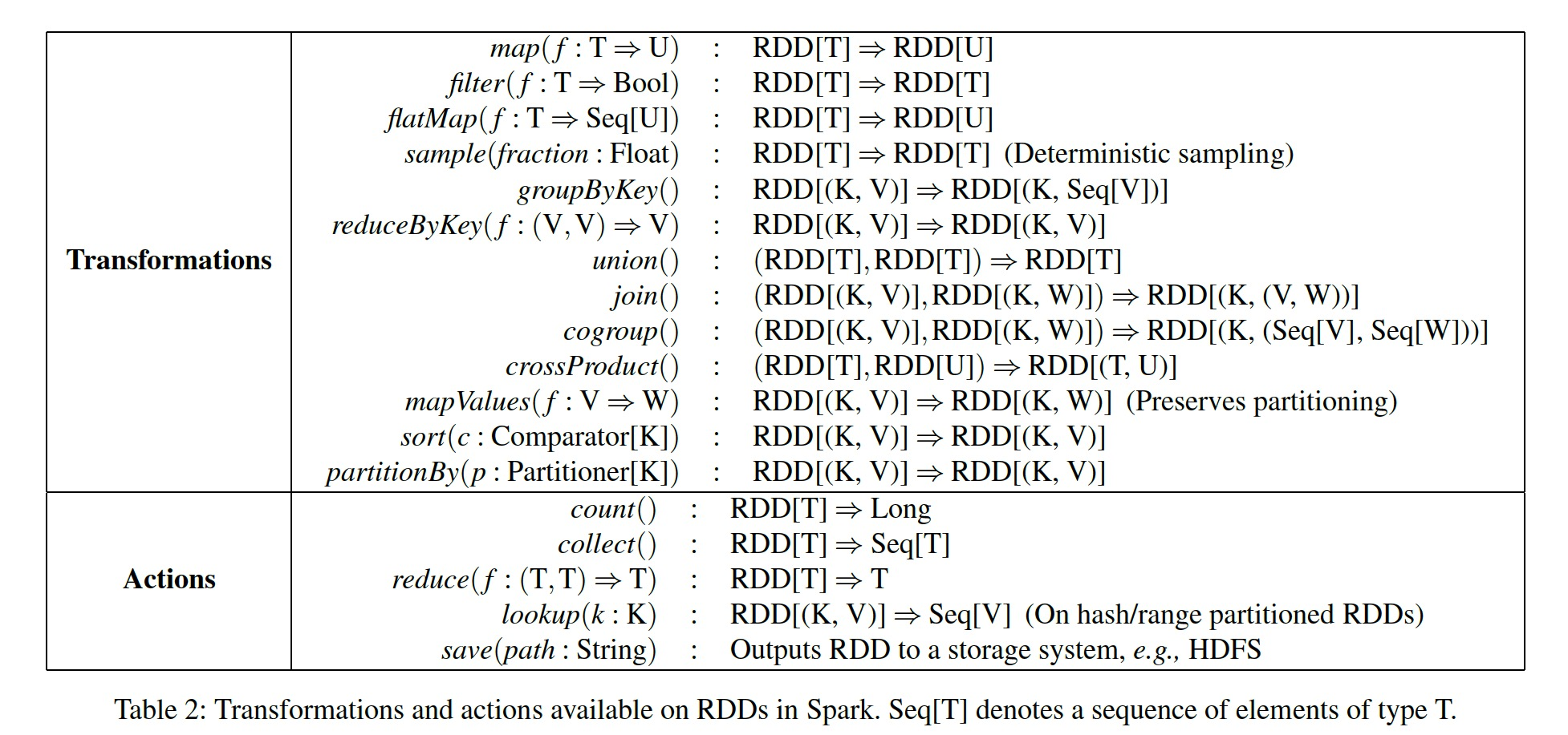 rdd-operators.png
Based on this, users can perform arbitrarily complex data processing. Physically, multiple datasets (nodes) and operators (edges) form a complex DAG (directed acyclic graph) execution topology:
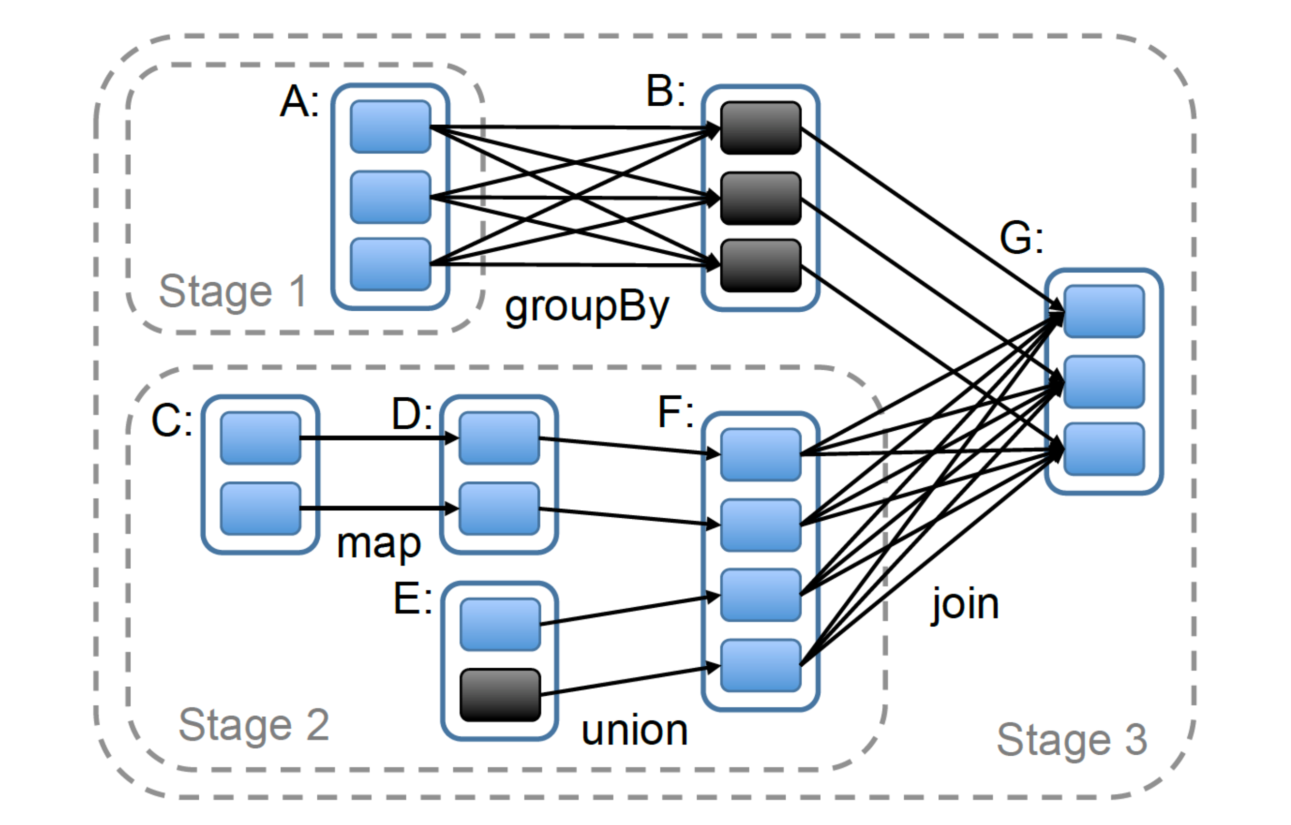 rdd-dag.png
Relational Databases
Relational databases are the culmination of data processing systems. On the one hand, they provide a powerful declarative query language — SQL — which balances flexibility and ease of use. On the other hand, they use compact, index-friendly storage internally, supporting efficient data query needs. Relational database systems integrate both computation and storage, and fully exploit the characteristics of hard drives and even networks (in the case of distributed databases), serving as a paragon of comprehensive utilization of computer resources. This article will not elaborate excessively on every aspect of relational database implementation, but will focus on the key points of this article — the standard dataset and composable operators.
The basic unit of data organization that relational databases provide to users is the relation, or table. In the SQL model, this is a strongly-typed two-dimensional table composed of rows and columns. Strong typing can be logically understood as requiring that the data stored in each cell must conform to the type definition of that column’s “header.” For this standard two-dimensional table, users can apply various relational algebra operators (selection, projection, Cartesian product).
After an SQL statement enters the RDBMS, it goes through parsing, validation, optimization, and is finally transformed into an operator tree for execution. The corresponding logical unit in the RDBMS is usually called the execution engine. Facebook Velox is a C++ library specifically targeting this niche.
Traditional execution engines often use the volcano model, a pull-based execution style. The basic concept is to organize operators in a tree structure, starting from the root node and recursively calling top-down, with operators returning data bottom-up at the granularity of rows or batches.

In recent years, the push-based style has gradually gained popularity; DuckDB and Velox both belong to this school. Similar to converting recursion into iteration, it goes bottom-up, computing from the leaf nodes and pushing results to the parent nodes until the root node. Each operator tree can be broken down into multiple operator pipelines that can execute in parallel (image source: Facebook Velox documentation)
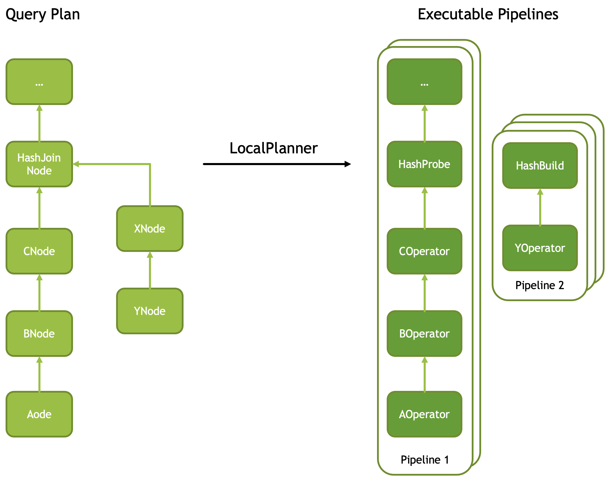 pipeline-break.png
If we rotate the above image clockwise by ninety degrees, we can see that its execution method is exactly the same as Spark’s. For more analysis of the Velox mechanism, you can refer to this article I wrote.
But whether push or pull, their abstractions of datasets and operators both conform to the theory proposed at the beginning of this article.
Summary
After examining the above four systems, we can see that data processing is, in a sense, a grand unification — first abstracting a normalized dataset, then providing a set of operations that can be applied to that dataset, and ultimately expressing users’ various data processing needs through composition.
This article is from my paid column on Xiaobot, “System Thinking Daily,” focusing on distributed systems, storage, and databases. It includes series on graph databases, code deep dives, high-quality English podcast translations, database learning, paper interpretations, and more. Welcome friends who enjoy my articles to subscribe 👉Column to support me; your support is very important for my continued creation of high-quality articles. Below is the current list of articles:
Graph Database Series
- 图数据库资料汇总
- 译: Factorization & Great Ideas from Database Theory
- Memgraph 系列(二):可串行化实现
- Memgraph 系列(一):数据多版本管理
- 【图数据库系列四】与关系模型的“缘”与“争”
- 【图数据库系列三】图的表示与存储
- 【图数据库系列二】 Cypher 初探
- 【图数据库系列一】属性图模型是啥、有啥不足 🔥
Databases
- 译:数据库五十年来研究趋势
- 译:数据库中的代码生成(Codegen in Databas…
- Facebook Velox 运行机制解析
- 分布式系统架构(二)—— Replica Placement
- 【好文荐读】DuckDB 中的流水线构建
- 译:时下大火的向量数据库,你了解多少?
- 数据处理的大一统——从 Shell 脚本到 SQL 引擎
- Firebolt:如何在十八个月内组装一个商业数据库
- 论文:NUMA-Aware Query Evaluation Framework 赏析
- 优质信息源:分布式系统、存储、数据库 🔥
- 向量数据库 Milvus 架构解析(一)
- ER 模型背后的建模哲学
- 什么是云原生数据库?
Storage
- 存储引擎概述和资料汇总 🔥
- 译:RocksDB 是如何工作的
- RocksDB 优化小解(二):Prefix Seek 优化
- RocksDB 优化小解(三):Async IO
- 大规模系统中使用 RocksDB 的一些经验
Code & Programming
- 影响我写代码的三个 “Code” 🔥
- Folly 异步编程之 futures
- 关于接口和实现
- C++ 私有函数的 override
- ErrorCode 还是 Exception ?
- Infra 面试之数据结构(一):阻塞队列
- 数据结构与算法(四):递归和迭代
Daily Database Learning Series
- 【每天学点数据库】Lecture #06:内存管理
- 【每天学点数据库】Lecture #05:数据压缩
- 【每天学点数据库】Lecture #05:负载类型和存储模型
- 【每天学点数据库】Lecture #04:数据编码
- 【每天学点数据库】Lecture #04:日志构型存储
- 【每天学点数据库】Lecture #03:Data Layout
- 【每天学点数据库】Lecture #03: Database and OS
- 【每天学点数据库】Lecture #03:存储层次体系
- 【每天学点数据库】Lecture #01:关系代数
- 【每天学点数据库】Lecture #01:关系模型
- 【每天学点数据库】Lecture #01:数据模型
Miscellaneous
- 数据库面试的几个常见误区 🔥
- 生活工程学(一):多轮次拆解🔥
- 系统中一些有趣的概念对
- 系统设计时的简洁和完备
- 工程经验的周期
- 关于“名字”拿来
- Cache 和 Buffer 都是缓存有什么区别?