DDIA Reading Notes (Chapter 2): Data Models and Query Languages

DDIA Reading Group: We will share chapter by chapter, combining my experience in distributed storage and databases in the industry with additional details. Sharing roughly every two weeks — welcome to join! The schedule and all transcripts are here. We have a corresponding distributed systems & database discussion group; notifications go out before each session. If you’d like to join, add me on WeChat: qtmuniao, briefly introduce yourself, and mention “Distributed Systems Group.”

Overview

This section revolves around two main concepts.

How to analyze a data model:

1. Basic considerations: the fundamental elements of data, and the relationships between elements (one-to-many, many-to-many).
2. Compare several common models: the (most popular) relational model, the (tree-like) document model, and the (highly flexible) graph model.
3. Schema patterns: strong schema (write-time constraints); weak schema (read-time parsing).

How to evaluate query languages:

1. How they relate to and match the data model.
2. Declarative vs. imperative.

Author: Muniao’s Notes https://www.qtmuniao.com/2022/04/16/ddia-reading-chapter2 Please cite the source when reposting

Data Model

A data model is an abstract model that organizes elements of data and standardizes how they relate to one another and to the properties of real-world entities.
—https://en.wikipedia.org/wiki/Data_model

Data model: how to organize data, how to standardize relationships, and how to connect with reality.

It determines both the way we build software (implementation) and the perspective from which we view problems (cognition).

The author opens by using different abstraction levels of computers to give an overall sense of generalized data models.

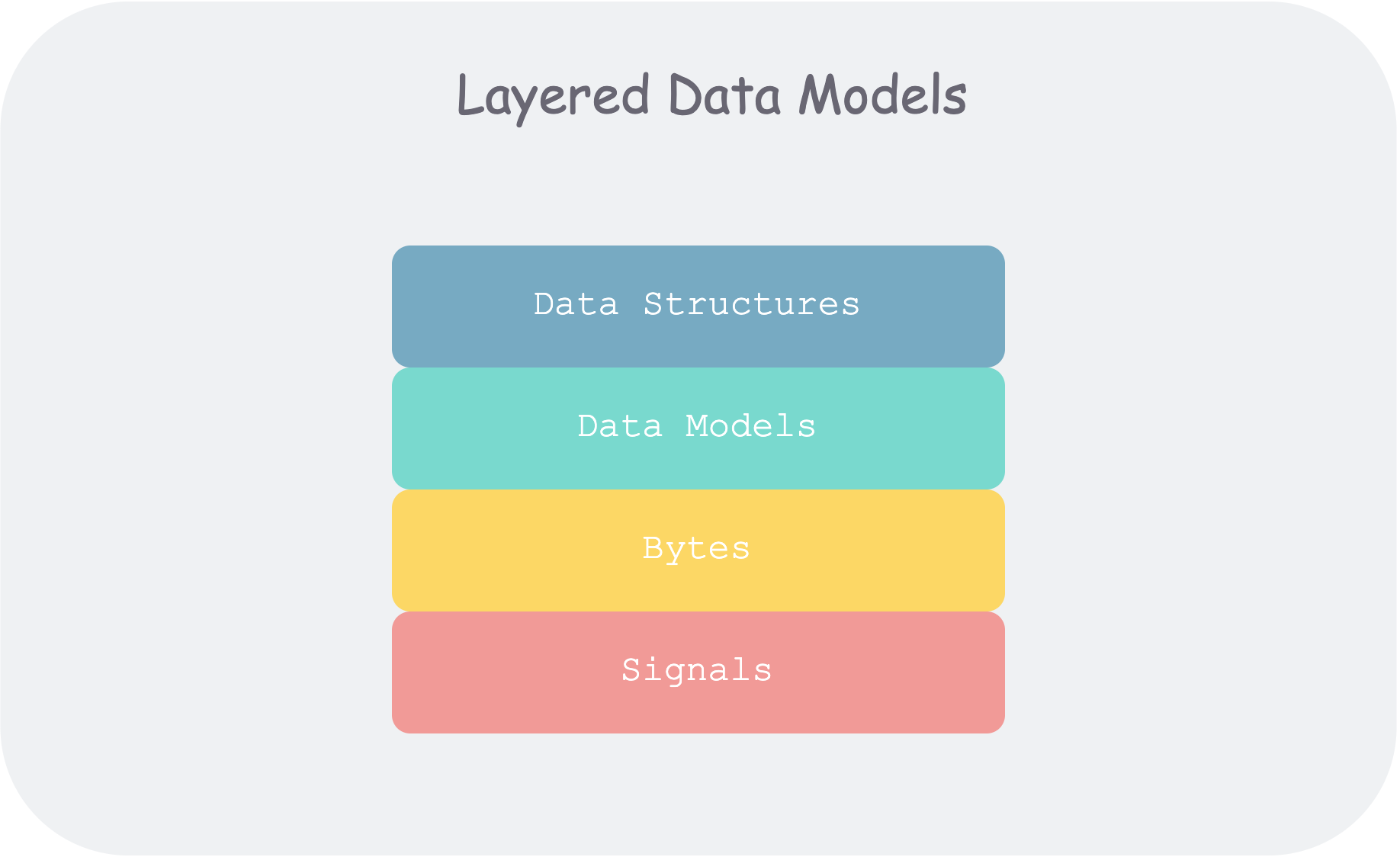
Most applications are built by progressively layering different data models.

ddia2-layered-data-models.png

The core question at each layer: how to model this layer using the interface of the layer below?

1. As an application developer, you abstract real-world problems into a set of objects, data structures, and APIs operating on them.
2. As a database administrator (DBA), to persist the above data structures, you need to express them using a general data model, such as XML/JSON in document databases, tables in relational databases, or graphs in graph databases.
3. As a database system developer, you need to organize the above data models into bytes in memory, on disk, or over the network, and provide various methods to manipulate data collections.
4. As a hardware engineer, you need to represent the byte stream as diode potentials (memory), magnetic poles in a field (disk), or light signals in optical fiber (network).

At each layer, by exposing a concise data model, we isolate and decompose the complexity of the real world.

This also illustrates that a good data model needs two characteristics:

1. Concise and intuitive.
2. Composable.

Chapter 2 first explores the relational model, the document model, and their comparison; then relevant query languages; and finally the graph model.

Relational Model vs. Document Model

Relational Model

The relational model is undoubtedly the most popular database model today.

The relational model was first proposed by Edgar Codd in 1969, and explained using “Codd’s 12 rules”. However, commercially available databases have basically failed to fully comply with them, so the term “relational model” later came to refer to this general class of databases. Its characteristics are:

1. Presents data to users as relations (e.g., two-dimensional tables containing rows and columns).
2. Provides relational operators to manipulate data sets.

Common Classifications

1. Transactional (TP): banking transactions, train tickets.
2. Analytical (AP): data reports, monitoring dashboards.
3. Hybrid (HTAP):

Many years after the birth of the relational model, although challengers emerged from time to time (such as the network model and hierarchical model of the 1970s and 1980s), no fundamentally new model capable of shaking its position ever appeared.

Until the last decade, with the proliferation of mobile internet, the explosive growth of data, and increasingly refined processing requirements, a blossoming of data models has been spurred.

The Birth of NoSQL

NoSQL (originally meaning Non-SQL, later reinterpreted as Not only SQL) is a general term for database management systems that differ from traditional relational databases. According to the DB-Engines ranking, the most popular NoSQL databases today are MongoDB, Redis, ElasticSearch, and Cassandra.

The driving factors include:

1. Handling larger datasets: greater scalability, higher throughput.
2. The rise of open source and free software: challenging the standards previously controlled by vendors.
3. Specialized query operations: things relational databases struggle to support, such as multi-hop analysis in graphs.
4. Stronger expressive power: the relational model is too rigid and restrictive.

The Object-Relational Mismatch

The core conflict lies in the nesting of object-oriented design versus the flatness of the relational model (a term I made up).

Of course, ORM frameworks can help us handle these matters, but it’s still somewhat inconvenient.

ddia2-bill-resume.png

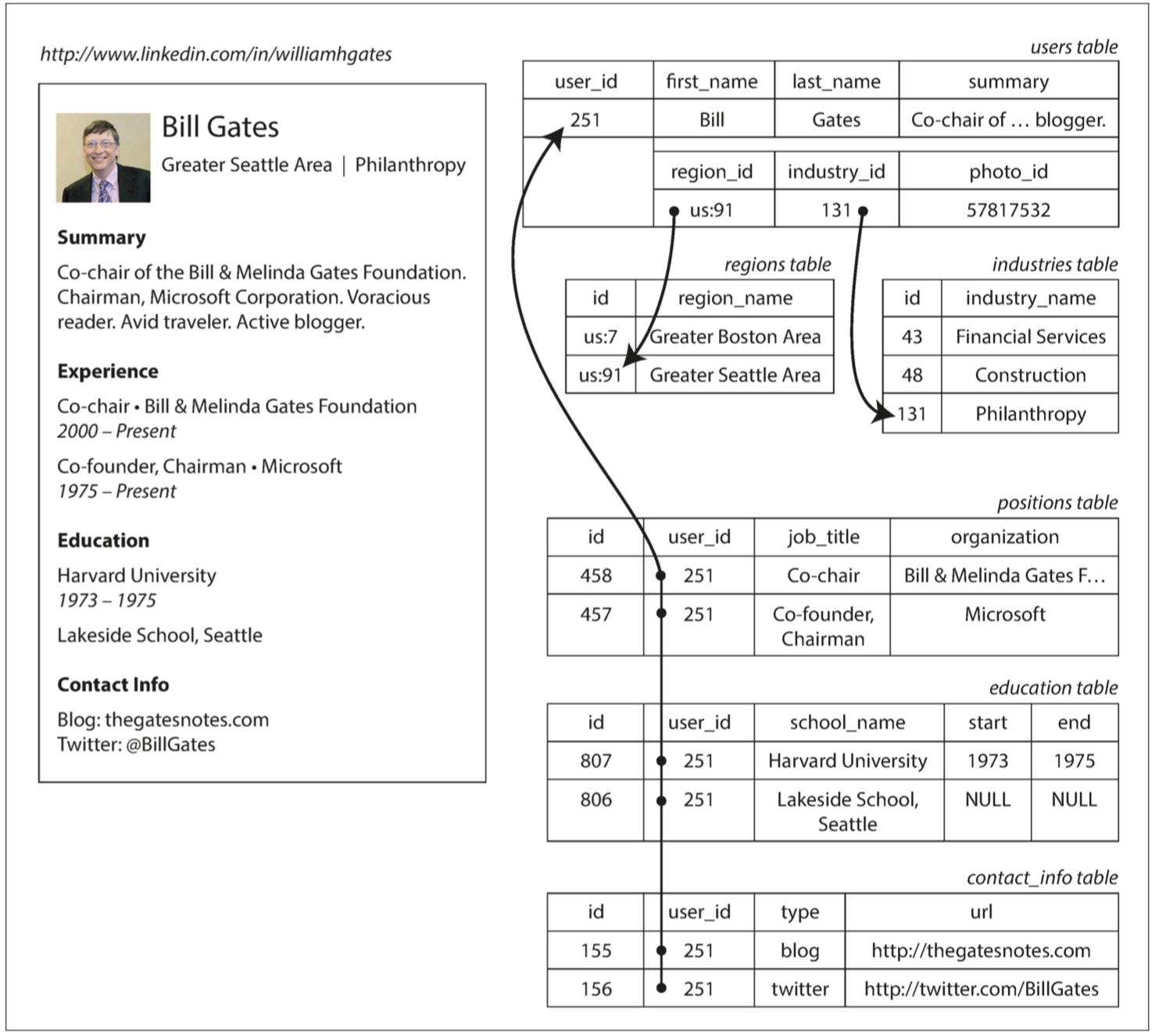
From another perspective, the relational model makes it difficult to intuitively represent one-to-many relationships. For example, on a resume, one person may have multiple education experiences and multiple work experiences.

Document model: leverages the natural nesting of JSON and XML.

Relational model: using the SQL model, positions and education must be split into separate tables, then linked via foreign keys in the user table.

In the resume example, the document model has several additional advantages:

1. Schema flexibility: fields can be dynamically added or removed, such as work experience.
2. Better locality: when all attributes of a person are accessed together, they are also stored together.
3. Structure conveys semantics: the implicit one-to-many tree-like relationship between a resume and contact info, education, career info, etc., can be explicitly expressed by JSON’s tree structure.

Many-to-One and Many-to-Many

This is an angle for comparing various data models.

When storing a region, why not store the plain string “Greater Seattle Area” directly, but instead store it as region_id → region name, with everywhere else referencing region_id?

1. Unified style: all places using the same concept have identical spelling and formatting.
2. Avoid ambiguity: there may be regions with the same name.
3. Ease of modification: if a region is renamed, we don’t need to modify every place that references it.
4. Localization support: if translating into other languages, only the name table needs translation.
5. Better search: lists can be associated with regions for hierarchical organization.

A similar concept: program to abstractions, not to details.

Regarding the choice between IDs and text, the author makes a point: IDs are meaningless to humans, and being meaningless means they won’t change as the real world changes in the future.

This needs to be considered when designing relational database tables, i.e., how to control duplication. Several normal forms exist to eliminate redundancy.

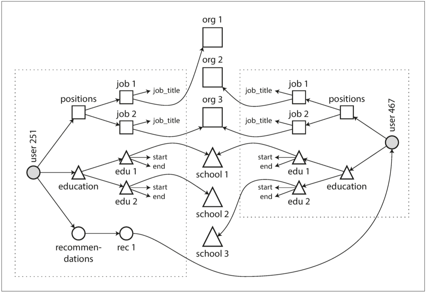
Document databases excel at handling one-to-many tree-like relationships but struggle with many-to-many graph-like relationships. If they don’t support Joins, the complexity of handling many-to-many relationships shifts from the database side to the application side.

For example, multiple users may have worked at the same organization. If we want to find people who attended the same school and worked at the same organization, and the database doesn’t support Joins, the application side would need to perform nested loops to Join.

ddia2-mul-to-mul.png

Document vs. Relational

1. For one-to-many relationships, document databases place nested data inside the parent node, rather than splitting it out into a separate table.
2. For many-to-one and many-to-many relationships, essentially both use foreign keys (document references) for indexing. Queries require joins or dynamic following.

Is the Document Model Repeating History?

Hierarchical Model

In the 1970s, IBM’s Information Management System (IMS).

A hierarchical database model is a data model in which the data are organized into a tree-like structure. The data are stored as records which are connected to one another through links. A record is a collection of fields, with each field containing only one value. The type of a record defines which fields the record contains. — wikipedia

Key points:

1. Tree-like organization; each child node is allowed only one parent node.
2. Nodes store data; nodes have types.
3. Nodes are connected using pointer-like links.

As can be seen, it is very similar to the document model, and therefore also struggles to solve many-to-many relationships and does not support Joins.

To address the limitations of the hierarchical model, various solutions were proposed, the most prominent being:

1. The relational model.
2. The network model.

Network Model

The network model is an extension of the hierarchical model: it allows a node to have multiple parent nodes. It was standardized by the Committee on Data Systems Languages (CODASYL), and is therefore also known as the CODASYL model.

Many-to-one and many-to-many can both be represented by paths. The only way to access a record is by traversing the chain of elements and links, which is called an access path. The difficulty is akin to navigating in n-dimensional space.

Memory was limited, so traversal paths had to be strictly controlled. And because the database’s topological structure had to be known in advance, this meant writing large amounts of application-specific code for different applications.

Relational Model

In the relational model, data is organized into tuples, which are then collected into relations; in SQL these correspond to rows and tables.

• Ever wonder why it’s called the relational model when it looks more like a table model?

  A table is just one implementation.

  The term “relation” comes from set theory, referring to a subset of the Cartesian product of several sets.

  R ⊆ (D1×D2×D3 ··· ×Dn)

  (Relation is denoted by R, attributes by Ai, and the domain of attributes by Di.)

Its main purpose and contribution is to provide a declarative way to describe data and construct queries.

That is, compared to the network model, the relational model decouples query statements from execution paths, with a query optimizer automatically deciding execution order and which indexes to use — decoupling logic from implementation.

For example: if you want to query your dataset in a new way, you only need to create an index on the new field. Then at query time, you don’t need to change your application code; the query optimizer will dynamically choose the available indexes.

Document vs. Relational

Choose the data model based on data characteristics.

	Document	Relational
Corresponding relationships	Data has natural one-to-many, tree-like nesting relationships, such as resumes.	Through foreign keys + Joins, can handle many-to-one and many-to-many relationships.
Code simplification	If data has a document structure, the document model is naturally suitable; using the relational model makes modeling tedious and access complex. But nesting shouldn’t be too deep, because access paths can only be manually specified or range-scanned.	Primary keys, indexes, conditional filtering.
Join support	Poor Join support.	Reasonable support, but Join implementation has many difficulties.
Schema flexibility	Weak schema, supports dynamically adding fields.	Strong schema; modifying the schema is costly.
Access locality	1. Accessing an entire document at once is efficient. 2. Accessing only part of a document is poor.	Scattered across multiple tables.

For highly interconnected datasets, using the document model feels awkward, using the relational model is acceptable, and using the graph model is the most natural.

Schema Flexibility in Document Models

Saying document databases are schemaless is not quite accurate; a more fitting description is schema-on-read.

Data Model		Programming Language		Performance & Space
schema-on-read	No validation on write; dynamic parsing on read.	Weakly typed	Dynamic, parsed at runtime	Dynamic parsing on read, poorer performance. Types cannot be determined at write time; space utilization is poor due to lack of alignment.
schema-on-write	Validated on write; data aligned to schema.	Strongly typed	Static, determined at compile time	Better performance and space usage.

Characteristics of document database use cases:

1. There are many types of data, but it’s not appropriate to put each in a separate table.
2. Data types and structures are determined externally; you have no control over data changes.

Data Locality at Query Time

If you need all contents of a document at the same time, storing the document sequentially will be more efficient.

But if you only need to access certain fields, the document still needs to be fully loaded.

However, exploiting this locality is not limited to document databases. Different databases will adjust physical data distribution for different scenarios to adapt to the locality of common access patterns.

• For example, in Spanner, tables can be declared as embedded into parent tables — common association inlining.
• HBase and Cassandra use column families to cluster data — analytical.
• In graph databases, vertices and their outgoing edges are stored on the same machine — graph traversal.

Convergence of Relational and Document Models

• MySQL and PostgreSQL have started supporting JSON.

  Native JSON support can be understood as: MySQL understands the JSON format. Like a Date format, a field can be treated as JSON, a sub-field can be modified, and indexes can be built on sub-fields.

• RethinkDB supports relational-link Joins in queries.

Codd: nonsimple domains, where values in a record can be not only simple types (numbers, strings) but also a nested relation (table). This is much like SQL’s support for XML and JSON.

Data Query Languages

Retrieve all shark-like animals from the animals table.

function getSharks() { var sharks = [];
  for (var i = 0; i < animals.length; i++) { 
    if (animals[i].family === "Sharks") {
      sharks.push(animals[i]);
    }
  }
  return sharks; 
}

SELECT * FROM animals WHERE family = 'Sharks';

	Declarative Language	Imperative Language
Concept	Describes control logic rather than execution flow.	Describes the execution process of commands, using a series of statements to continuously change state.
Examples	SQL, CSS, XSL	IMS, CODASYL, general-purpose languages like C, C++, JS
Abstraction level	High	Low
Coupling degree	Decoupled from implementation. Query engine performance can be continuously optimized.	Deeply coupled with implementation.
Parsing & Execution	Lexical analysis → Syntax analysis → Semantic analysis Generate execution plan → Execution plan optimization	Lexical analysis → Syntax analysis → Semantic analysis Intermediate code generation → Code optimization → Target code generation
Multi-core parallelism	Declarative has more multi-core potential, giving more runtime optimization space.	Imperative specifies code execution order, leaving less room for compile-time optimization.

• Q: What are the advantages of imperative languages relative to declarative languages?
  1. When the target becomes complex, declarative languages lack expressive power.
  2. Languages implementing the imperative paradigm are often not as strictly separated from declarative ones; through reasonable abstraction and programming paradigms (functional), code can balance expressiveness and clarity.

Beyond Databases: Declarative in the Web

Requirement: selected page background turns blue.

<ul>
  <li class="selected">
    <p>Sharks</p> 
    <ul>
      <li>Great White Shark</li> 
      <li>Tiger Shark</li> 
      <li>Hammerhead Shark</li>
    </ul>
  </li>
  <li> 
    <p>Whales</p>
    <ul>
      <li>Blue Whale</li>
      <li>Humpback Whale</li>
      <li>Fin Whale</li>
    </ul> 
  </li>
</ul>

If using CSS, you only need (CSS selector):

li.selected > p { 
  background-color: blue;
}

If using XSL, you only need (XPath selector):

<xsl:template match="li[@class='selected']/p"> 
  <fo:block background-color="blue">
    <xsl:apply-templates/>
  </fo:block>
</xsl:template>

But if using JavaScript (without the above selector libraries):

var liElements = document.getElementsByTagName("li"); 
for (var i = 0; i < liElements.length; i++) {
  if (liElements[i].className === "selected") { 
    var children = liElements[i].childNodes; 
    for (var j = 0; j < children.length; j++) {
      var child = children[j];
      if (child.nodeType === Node.ELEMENT_NODE && child.tagName === "P") {
        child.setAttribute("style", "background-color: blue");
      }
    } 
  }
}

MapReduce Queries

Google’s MapReduce Model

1. Borrowed from functional programming.
2. A fairly simple programming model, or atomic abstraction, that is somewhat insufficient today.
3. But in the barbaric era before big data processing tools were abundant (before 2003), the framework proposed by Google was quite pioneering.

Untitled

MongoDB’s MapReduce Model

MongoDB’s MapReduce is a hybrid data model between:

1. Declarative: users don’t need to explicitly define dataset traversal, shuffle processes, etc.
2. Imperative: users still need to define the execution process for individual records.

Requirement: count the number of shark observations per month.

Query Statements:

PostgreSQL

SELECT date_trunc('month', observation_timestamp) AS observation_month, 
  sum(num_animals) AS total_animals
FROM observations
WHERE family = 'Sharks' GROUP BY observation_month;

MongoDB

db.observations.mapReduce(
  function map() { // 2. Execute map on all matching docs
    var year = this.observationTimestamp.getFullYear();
    var month = this.observationTimestamp.getMonth() + 1; 
    emit(year + "-" + month, this.numAnimals); // 3. Output a kv pair
  },
  function reduce(key, values) { // 4. Aggregate by key
    return Array.sum(values);    // 5. Sum values with the same key
  },
  {
    query: { family: "Sharks" }, // 1. Filter
    out: "monthlySharkReport"    // 6. Reduce result set
  } 
);

When executed, the above statement goes through: filter → traverse and execute map → aggregate output by key (shuffle) → reduce aggregated data → output result set.

Some characteristics of MapReduce:

1. Requires Map and Reduce to be pure functions. That is, no side effects; executing any number of times, anywhere, in any order, for the same input, always produces the same output. Therefore, it’s easy to schedule concurrently.
2. A very low-level but powerfully expressive programming model. Higher-level query languages like SQL can be built on top of it, such as Hive.

But note:

1. Not all distributed SQL implementations are based on MapReduce.
2. MapReduce is not the only one that allows embedding general-purpose language (e.g., JS) modules.
3. MapReduce has a certain learning cost; you need to be familiar with its execution logic to make the two functions work closely together.

MongoDB 2.2+ evolved version, aggregation pipeline:

db.observations.aggregate([
  { $match: { family: "Sharks" } },
  { $group: {
    _id: {
      year:  { $year:  "$observationTimestamp" },
      month: { $month: "$observationTimestamp" }
    },
    totalAnimals: { $sum: "$numAnimals" } }}
]);

Graph-Like Data Models

• When is the document model suitable?

  When your dataset contains a large number of one-to-many relationships.

• When is the graph model suitable?

  When your dataset contains a large number of many-to-many relationships.

Basic Concepts

The basic concepts of graph data models generally include three things: vertices, edges, and properties attached to both.

Common scenarios that can be modeled with graphs:

Example	Modeling	Application
Social graph	People are vertices, follow relationships are edges.	Six degrees of separation, feed recommendation.
Web	Web pages are vertices, links are edges.	PageRank
Road network	Transportation hubs are vertices, railways/highways are edges.	Route planning, shortest-path navigation.
Money laundering	Accounts are vertices, transfer relationships are edges.	Detecting cycles.
Knowledge graph	Concepts are vertices, associations are edges.	Heuristic Q&A.

• Homogeneous and heterogeneous data

  Vertices in a graph can all be of the same type, but they can also be of different types — and the latter is even more powerful.

This section will use the following figure as an example. It represents a married couple: Lucy from Idaho, USA, and Alain from France. They are married and live in London.

Untitled

There are multiple ways to model a graph:

1. Property graph: more mainstream, e.g., Neo4j, Titan, InfiniteGraph.
2. Triple-store: e.g., Datomic, AllegroGraph.

Property Graph (PG, Property Graphs)

Vertices (vertices, nodes, entities)	Edges (edges, relations, arcs)
Globally unique ID	Globally unique ID
Set of outgoing edges	Start vertex
Set of incoming edges	End vertex
Property set (represented as kv pairs)	Property set (represented as kv pairs)
Type indicating vertex type?	Label indicating edge type

• Q: One puzzling point — why does the book’s definition of PG vertices not include Type?

  If the data is heterogeneous, there should be one; is it perhaps marking different types through different properties?

If it doesn’t feel intuitive, we can use familiar SQL semantics to construct a graph model, as shown below. (Facebook’s TAO paper uses MySQL as its single-machine storage engine.)

// Vertex table
CREATE TABLE vertices (
  vertex_id integer PRIMARYKEY, properties json
);

// Edge table
CREATE TABLE edges (
  edge_id integer PRIMARY KEY,
  tail_vertex integer REFERENCES vertices (vertex_id), 
  head_vertex integer REFERENCES vertices (vertex_id),
  label text,
  properties json
);

// Reverse index on vertices, used during graph traversal. Given a vertex, find all its incoming and outgoing edges.
CREATE INDEX edges_tails ON edges (tail_vertex);
CREATE INDEX edges_heads ON edges (head_vertex);

Graphs are a very flexible modeling approach:

1. Edges can be inserted between any two vertices without any schema restrictions.
2. For any vertex, its incoming and outgoing edges can be found efficiently (think: how to be efficient?), enabling graph traversal.
3. Multiple labels are used to mark different types of edges (relationships).

Compared to relational data, heterogeneous types of data and relationships can be stored in the same graph, giving graphs tremendous expressive power!

This expressive power includes, according to the example in the figure:

1. For the same concept, different structures can be used. Such as administrative divisions in different countries.
2. For the same concept, different granularities can be used. Such as Lucy’s current residence and birthplace.
3. Can evolve very naturally.

Accommodating heterogeneous data in a single graph, graph traversal can easily accomplish operations that would require multiple Joins in a relational database.

Cypher Query Language

Cypher is a query language created by Neo4j.

The names Cypher and Neo likely both come from The Matrix. Think Oracle.

A major characteristic of Cypher is its readability, especially when expressing path patterns.

Combining with the previous figure, here is an example of a Cypher insert statement:

CREATE
  (NAmerica:Location {name:'North America', type:'continent'}),
  (USA:Location      {name:'United States', type:'country'  }),
  (Idaho:Location    {name:'Idaho',         type:'state'    }),
  (Lucy:Person       {name:'Lucy' }),
  (Idaho) -[:WITHIN]->  (USA)  -[:WITHIN]-> (NAmerica),
  (Lucy)  -[:BORN_IN]-> (Idaho)

If we want to perform a query like this: find the names of all people who emigrated from the United States to Europe.

Translated into graph language: given the conditions, BORN_IN points to a location in the United States, and LIVES_IN points to a location in Europe; find all vertices satisfying the above conditions and return their name properties.

In Cypher, this can be expressed as:

MATCH
  (person) -[:BORN_IN]->  () -[:WITHIN*0..]-> (us:Location {name:'United States'}),
  (person) -[:LIVES_IN]-> () -[:WITHIN*0..]-> (eu:Location {name:'Europe'})
RETURN person.name

Notice:

1. Vertices (), edges -[]→, labels/types :, properties {}.
2. Name binding or variables: person
3. Zero-to-many wildcard: *0...

As is characteristic of declarative query languages, you only need to describe the problem without worrying about the execution process. But unlike SQL, which is based on relational algebra, Cypher is more like regular expressions.

Implementation details such as BFS, DFS, or pruning don’t need to be concerned with.

Using SQL for Graph Queries

We saw earlier that SQL can be used to store vertices and edges to represent a graph.

Can SQL be used for graph queries?

Oracle’s PGQL:

CREATE PROPERTY GRAPH bank_transfers
     VERTEX TABLES (persons KEY(account_number))
     EDGE TABLES(
                  transactions KEY (from_acct, to_acct, date, amount)
                  SOURCE KEY (from_account) REFERENCES persons
                  DESTINATION KEY (to_account) REFERENCES persons
                  PROPERTIES (date, amount)
       )

One difficulty is how to express graph patterns, such as multi-hop queries, which in SQL corresponds to joins of uncertain number:

() -[:WITHIN*0..]-> ()

This can be satisfied using recursive common table expressions in SQL:1999 (supported by PostgreSQL, IBM DB2, Oracle, and SQL Server). However, it is quite verbose and clumsy.

Triple-Stores and SPARQL

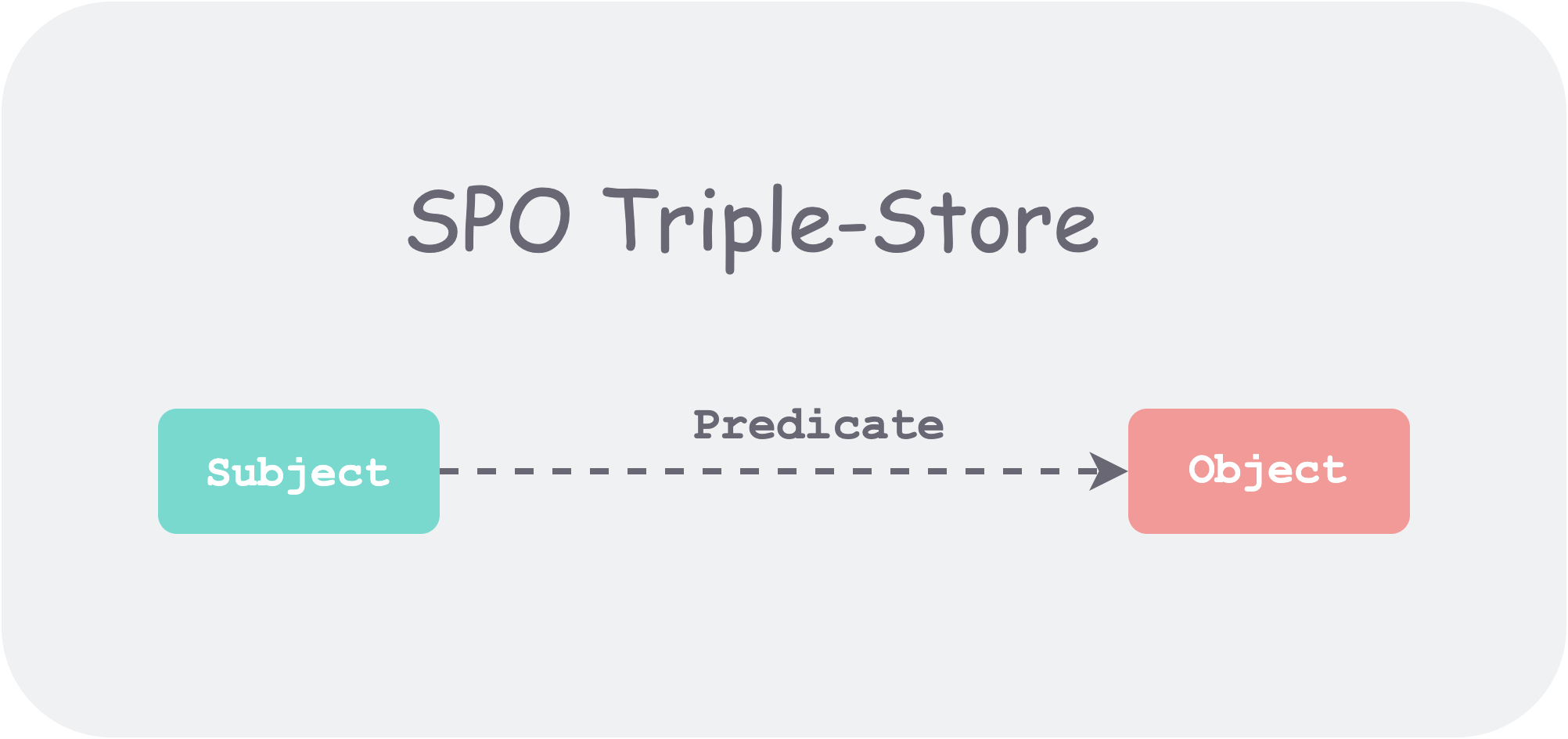
Triple-Stores can be understood as triple storage, i.e., storing graphs as triples.

ddia2-triple-store.png

Their meanings are as follows:

Subject	Corresponds to a vertex in the graph.
Object	1. An atomic value, such as a string or number. 2. Another Subject.
Predicate	1. If Object is atomic, then <Predicate, Object> corresponds to a kv pair attached to the vertex. 2. If Object is another Subject, then Predicate corresponds to an edge in the graph.

Using the same example above, expressed in Turtle triples (a Triple-Stores syntax):

@prefix : <urn:example:>.
_:lucy     a       :Person.
_:lucy     :name   "Lucy".
_:lucy     :bornIn _:idaho.
_:idaho    a       :Location.
_:idaho    :name   "Idaho".
_:idaho    :type   "state".
_:idaho    :within _:usa.
_:usa      a       :Location
_:usa      :name   "United States"
_:usa      :type   "country".
_:usa      :within _:namerica.
_:namerica a       :Location.
_:namerica :name   "North America".
_:namerica :type   "continent".

A more compact notation:

@prefix : <urn:example:>.
_:lucy     a: Person;   :name "Lucy";          :bornIn _:idaho
_:idaho    a: Location; :name "Idaho";         :type "state";     :within _:usa.
_:usa      a: Location; :name "United States"; :type "country";   :within _:namerica.
_:namerica a :Location; :name "North America"; :type "continent".

The Semantic Web

Proposed by Tim Berners-Lee, father of the World Wide Web, in 1998; the predecessor of knowledge graphs. Its purpose is to structure resources on the network so that computers can understand data on the web. That is, not as text, binary streams, etc., but through some standard of structured, interconnected data.

Semantics: provide a unified way to describe and structure all resources (machine-readable).

Web: connect all resources.

Below is the Semantic Web Stack:

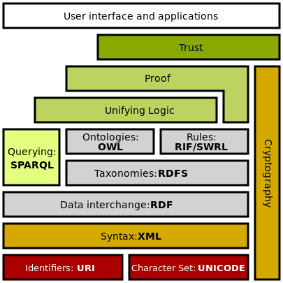ddia2-rdf.png

Among them, RDF (Resource Description Framework) provides a standard for structuring data on the web. Any resource published to the web (text, images, video, web pages) can be understood by computers in a unified form. That is, resource consumers don’t need to deeply learn to extract the semantics of resources; instead, resource providers actively provide their resource semantics through RDF.

It feels somewhat idealistic, but the Internet and open-source communities have developed precisely through this idealism and spirit of sharing!

Although the Semantic Web did not take off, its intermediate data exchange format RDF, and the SPO triples (Subject-Predicate-Object) it defines, constitute a very useful data model — the Triple-Stores mentioned above.

RDF Data Model

The Turtle language (SPO triples) mentioned above is a simple and readable way to describe RDF data. RDF can also be represented based on XML, but it is much more redundant and harder to read (nesting is too deep):

<rdf:RDF xmlns="urn:example:"
  xmlns:rdf="http://www.w3.org/1999/02/22-rdf-syntax-ns#">
  <Location rdf:nodeID="idaho"> 
    <name>Idaho</name>
    <type>state</type>
    <within>
      <Location rdf:nodeID="usa">
        <name>United States</name>
        <type>country</type>
        <within>
          <Location rdf:nodeID="namerica"> 
            <name>North America</name>
            <type>continent</type>
          </Location>
        </within>
      </Location>
    </within>
  </Location>
  <Person rdf:nodeID="lucy">
    <name>Lucy</name>
    <bornIn rdf:nodeID="idaho"/>
  </Person>
</rdf:RDF>

To standardize and remove ambiguity, some points that look rather strange: whether subject, predicate, or object, all are defined by URIs, such as:

lives_in would be represented as <http://my-company.com/namespace#lives_in>

The prefix is just a namespace, making the definition unique and accessible on the network. Of course, a simplified approach is to declare a common prefix in the file header.

SPARQL Query Language

With the Semantic Web, there naturally needs to be a traversal and query language within it, leading to RDF’s query language: SPARQL Protocol and RDF Query Language, pronounced “sparkle.”

PREFIX : <urn:example:>
SELECT ?personName WHERE {
  ?person :name ?personName.
  ?person :bornIn  / :within* / :name "United States".
  ?person :livesIn / :within* / :name "Europe".
}

It is the predecessor of Cypher, so the structure looks very similar:

(person) -[:BORN_IN]-> () -[:WITHIN*0..]-> (location)   # Cypher
?person   :bornIn /        :within*        ?location.   # SPARQL

But SPARQL does not distinguish between edges and properties; both use Predicates.

(usa {name:'United States'})   # Cypher
?usa :name "United States".    # SPARQL

Although the Semantic Web did not successfully land, its technology stack influenced later knowledge graphs and graph query languages.

Graph Model and Network Model

Is the graph model just old wine in new bottles for the network model?

No, they differ in many important ways.

Model	Graph Model	Network Model
Connection method	Edges can exist between any two vertices.	Specifies nesting constraints.
Record lookup	1. Use global ID. 2. Use property indexes. 3. Use graph traversal.	Can only use path queries.
Ordering	Vertices and edges are unordered.	Records’ children are ordered sets; insertion needs to consider the cost of maintaining order.
Query language	Can be both imperative and declarative.	Imperative.

Query Language Predecessor: Datalog

A bit like triple-store, but with the order changed: (subject, predicate, object) → predicate(subject, object).
The previous data represented in Datalog:

name(namerica, 'North America').
type(namerica, continent).

name(usa, 'United States').
type(usa, country).
within(usa, namerica).

name(idaho, 'Idaho').
type(idaho, state).
within(idaho, usa).

name(lucy, 'Lucy').
born_in(lucy, idaho).

Querying for people who migrated from the United States to Europe can be expressed as:

within_recursive(Location, Name) :- name(Location, Name). /* Rule 1 */
within_recursive(Location, Name) :- within(Location, Via), /* Rule 2 */ 
                                    within_recursive(Via, Name).

migrated(Name, BornIn, LivingIn) :- name(Person, Name), /* Rule 3 */ 
                                    born_in(Person, BornLoc),
                                    within_recursive(BornLoc, BornIn),
                                    lives_in(Person, LivingLoc),
                                    within_recursive(LivingLoc, LivingIn).
?- migrated(Who, 'United States', 'Europe'). /* Who = 'Lucy'. */

1. In the code, elements starting with an uppercase letter are variables; strings, numbers, or elements starting with a lowercase letter are constants. The underscore (_) is called an anonymous variable.
2. Basic Predicates can be used to define custom Predicates, similar to using basic functions to define custom functions.
3. Multiple predicate expressions connected by commas represent an AND relationship.

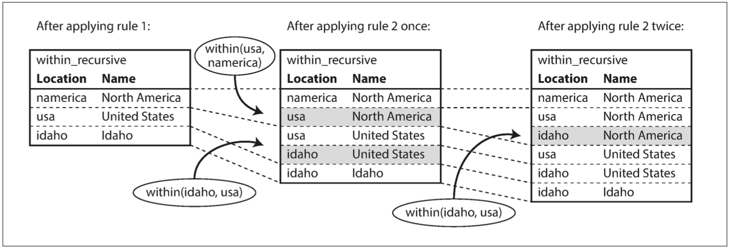ddia2-triple-store-query.png

Set-based logical operations:

1. Select qualifying sets from the basic data subset.
2. Apply rules to expand the original set.
3. If recursion is possible, recursively exhaust all possibilities.

Prolog (short for Programming in Logic) is a logic programming language. It is built on the theoretical foundation of logic.

References

1. Declarative vs. Imperative language: https://lotabout.me/2020/Declarative-vs-Imperative-language/
2. SimmerChan Zhihu column, knowledge graph, semantic web, RDF: https://www.zhihu.com/column/knowledgegraph
3. Why is MySQL called the “relational” model: https://zhuanlan.zhihu.com/p/64731206

---

我是青藤木鸟，一个喜欢摄影、专注大规模数据系统的程序员，欢迎关注我的公众号：“木鸟杂记”，有更多的分布式系统、存储和数据库相关的文章，欢迎关注。 关注公众号后，回复“资料”可以获取我总结一份分布式数据库学习资料。 回复“优惠券”可以获取我的大规模数据系统付费专栏《系统日知录》的八折优惠券。

我们还有相关的分布式系统和数据库的群，可以添加我的微信号：qtmuniao，我拉你入群。加我时记得备注：“分布式系统群”。 另外，如果你不想加群，还有一个分布式系统和数据库的论坛（点这里），欢迎来玩耍。