DDIA Reading Club: I will share chapter by chapter, adding some details based on my experience in distributed storage and databases in industry. Sharing roughly every two weeks—welcome to join! The schedule and all transcripts are here. We have a corresponding distributed systems & databases discussion group, and I will notify in the group before each session. If you’d like to join, add my WeChat: qtmuniao, briefly introduce yourself, and note: distributed systems group.

Chapter 2 discussed the upper-level abstractions: data models and query languages.
This chapter goes a bit deeper, focusing on how databases handle queries and storage at the low level. There is a logical chain here:

Use case → Query type → Storage format.

Author: 木鸟杂记 https://www.qtmuniao.com/2022/04/16/ddia-reading-chapter3-part1. Please indicate the source when reposting.

Query types are mainly divided into two categories:

Engine Type	Request Volume	Data Volume	Bottleneck	Storage Format	Users	Example Scenarios	Example Products
OLTP	Relatively frequent, focused on online transactions	Both total and per-query volumes are relatively small	Disk Seek	Mostly row-oriented	Relatively common, mostly used by general applications	Bank transactions	MySQL
OLAP	Relatively infrequent, focused on offline analytics	Both total and per-query volumes are relatively huge	Disk Bandwidth	Column-oriented is gaining popularity	Mostly business users	Business analytics	ClickHouse

Among these, on the OLTP side, commonly used storage engines fall into two schools:

School	Main Characteristics	Basic Idea	Representatives
Log-structured	Only appends allowed; all modifications appear as file appends and whole-file additions/deletions	Turn random writes into sequential writes	Bitcask, LevelDB, RocksDB, Cassandra, Lucene
Update-in-place	Modifies disk data at the granularity of a page	Page-oriented, search tree	B-tree family, all mainstream relational databases and some non-relational databases

In addition, for OLTP, we also explore common indexing methods and a special type of database—the in-memory database.

For data warehouses, this chapter analyzes their main differences from OLTP. Data warehouses mainly focus on aggregation queries that need to scan very large amounts of data; at this point, indexes are relatively less useful. What needs to be considered are storage costs, bandwidth optimization, etc., which leads to columnar storage.

Underlying Data Structures That Drive Databases

This section starts from a shell script, to a fairly simple but usable storage engine Bitcask, then leads to LSM-tree—they all belong to the log-structured category. Then it turns to another school of storage engines—the B-tree family, followed by a brief comparison. Finally, it explores an indispensable structure in storage: indexes.

First, let’s look at the “simplest” database in the world, composed of two Bash functions:

#!/bin/bash
db_set () {
  echo "$1,$2" >> database
}

db_get () {
  grep "^$1," database | sed -e "s/^$1,//" | tail -n 1
}

These two functions implement a string-based KV store (only supporting get/set, not delete):

$ db_set 123456 '{"name":"London","attractions":["Big Ben","London Eye"]}' 
$ db_set 42 '{"name":"San Francisco","attractions":["Golden Gate Bridge"]}'
$ db_get 42
{"name":"San Francisco","attractions":["Golden Gate Bridge"]}

Let’s analyze why it works, which also reflects the most basic principles of log-structured storage:

set: append a KV pair to the end of the file.
get: match all keys, return the value from the last (i.e., latest) KV pair.

It can be seen: writes are very fast, but reads require a full scan line by line, which is much slower. A typical trade-off of read for write. To speed up reads, we need to build an index: an additional data structure that allows lookups based on certain fields.

Indexes are built from the original data solely to speed up lookups. Therefore, indexes consume some extra space and insertion time (each insertion requires updating the index), i.e., trading space and writes for reads again.

This is the most common trade-off in database storage engine design and selection:

Appropriate storage formats can speed up writes (log-structured) but make reads very slow; they can also speed up reads (search trees, B-trees) but make writes slower.
To compensate for read performance, indexes can be built. But this sacrifices write performance and consumes extra space.

Storage formats are generally hard to change, but whether to build indexes or not is usually left to the user’s choice.

Hash Indexes

This section mainly focuses on the most basic KV index.

Following the example in the previous subsection, all data is sequentially appended to disk. To speed up queries, we build a hash index in memory:

Key is the query key.
Value is the starting position and length of the KV entry.

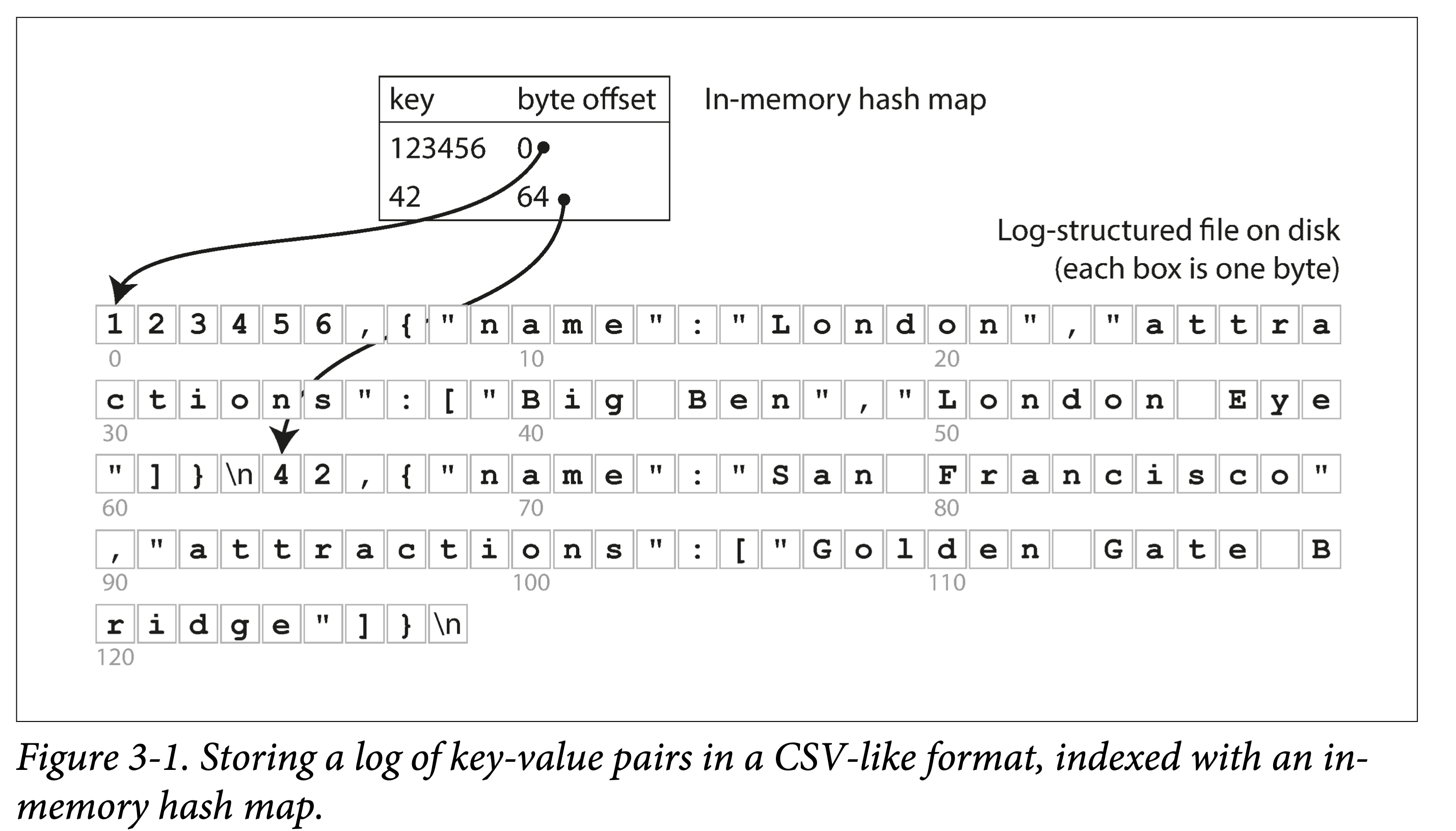ddia-3-1-hash-map-csv.png

It looks very simple, but this is exactly the basic design of Bitcask. The key is that it works (when the data volume is small, i.e., all keys can fit in memory): it can provide very high read and write performance:

Write: append to file.
Read: one memory lookup, one disk seek; if the data is already cached, the seek can also be saved.

If your key set is small (meaning it can all fit in memory), but each key is updated very frequently, then Bitcask is what you need. For example: frequently updated video view counts, where the key is the video URL and the value is the video view count.

But there is a very important problem: what if a single file keeps growing larger and disk space is insufficient?

When a file reaches a certain size, create a new file and make the original file read-only. At the same time, to reclaim the space wasted by multiple writes of the same key, read-only files can be compacted, rewriting old files to squeeze out the “water” (overwritten data) for garbage collection.

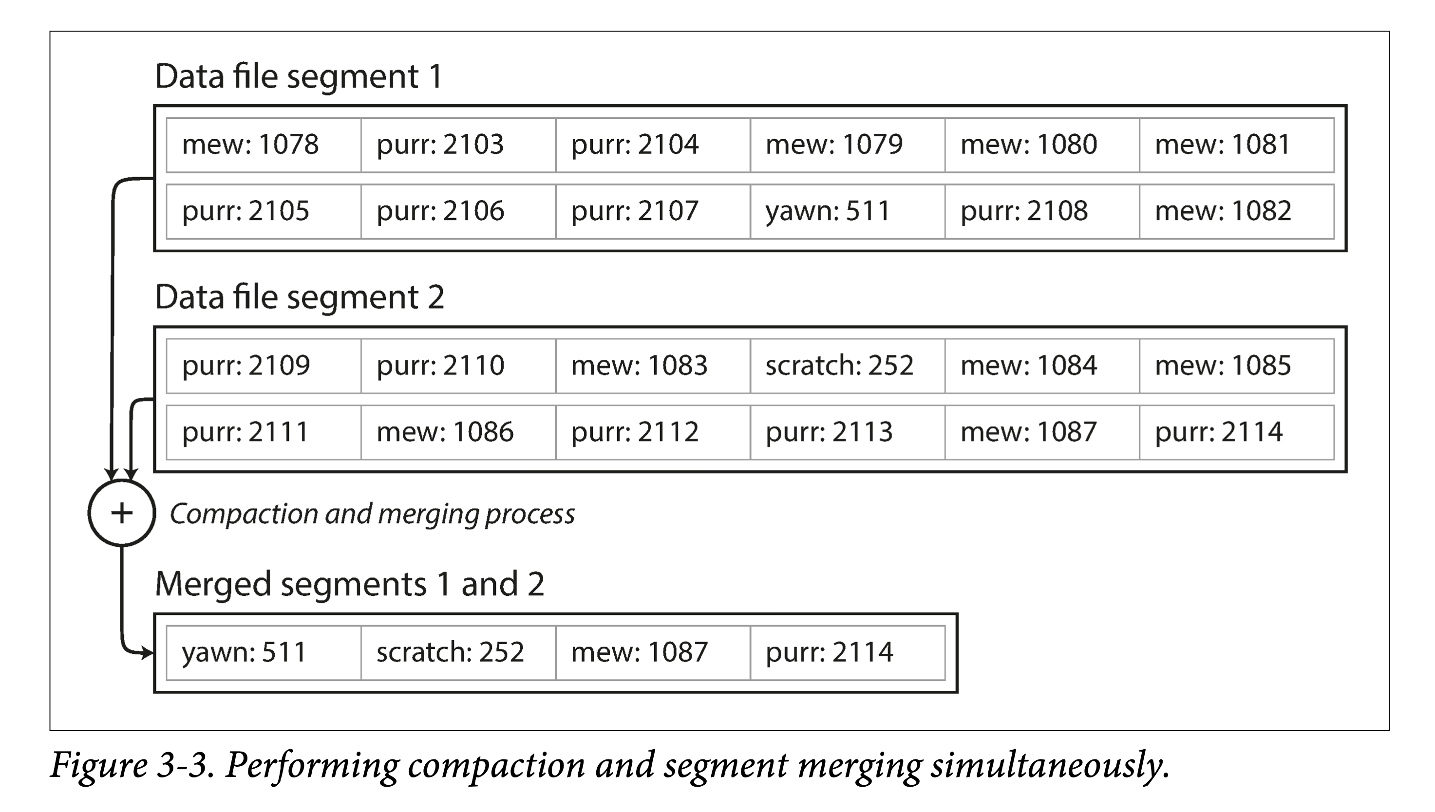ddia-3-3-compaction-sim.png

Of course, if we want to make it industrially usable, there are still many problems to solve:

File format. For logs, CSV is not a compact data format and wastes a lot of space. For example, length + record bytes could be used.
Record deletion. Previously only put/get were supported, but in practice delete also needs to be supported. But log-structured storage doesn’t support updates, so what to do? The usual approach is to write a special marker (such as a tombstone record) to indicate that the record has been deleted. It will be truly deleted during compaction later.
Crash recovery. When the machine restarts, the in-memory hash index will be lost. Of course, a full scan can be done to rebuild it, but a common small optimization is to persist the index entries together with the data file for each segment file, so that only the index entries need to be loaded upon restart.
Corrupted or partial writes. The system may crash at any time, which can cause records to be corrupted or partially written. To identify erroneous records, we need to add some checksum fields to recognize and skip such data. To skip partially written data, special characters are also needed to mark the boundaries between records.
Concurrency control. Since there is only one active (append) file, writes have only one natural degree of concurrency. But other files are immutable (read and new files are generated during compaction), so reads and compaction can be executed concurrently.

At first glance, log-based storage structures seem quite wasteful: updates and deletions require appending. But log-structured storage has several advantages that in-place update structures cannot achieve:

Replacing random writes with sequential writes. For both disks and SSDs, sequential writes are several orders of magnitude faster than random writes.
Simpler concurrency control. Since most files are immutable, it is easier to perform concurrent reads and compaction. There is also no need to worry about in-place updates causing old and new data to alternate.
Less internal fragmentation. Each compaction completely squeezes out garbage. But in-place updates leave some unusable space in pages.

Of course, in-memory hash indexes also have their limitations:

All keys must fit in memory. Once the data volume of keys exceeds memory size, this solution no longer works. Of course, you can design disk-based hash tables, but that would bring a large number of random writes.
Does not support range queries. Since keys are unordered, range queries require a full table scan.

The LSM-Tree and B+ trees discussed later can both partially avoid the above problems.

Think about it: how would they avoid these issues?

SSTables and LSM-Trees

This section progresses layer by layer, leading step by step from the SSTables format to the full picture of LSM-Trees.

For KV data, the BitCask storage structure mentioned earlier is:

Log segments on external storage.
A hash table in memory.

The data on external storage is formed by simple append writes and is not ordered by any field.

Suppose we add a constraint that these files are ordered by key. We call this format: SSTable (Sorted String Table).

What are the advantages of this file format?

Efficient data file merging. That is, merge sort of ordered files, sequential reads, sequential writes. What if the same key appears in different files?

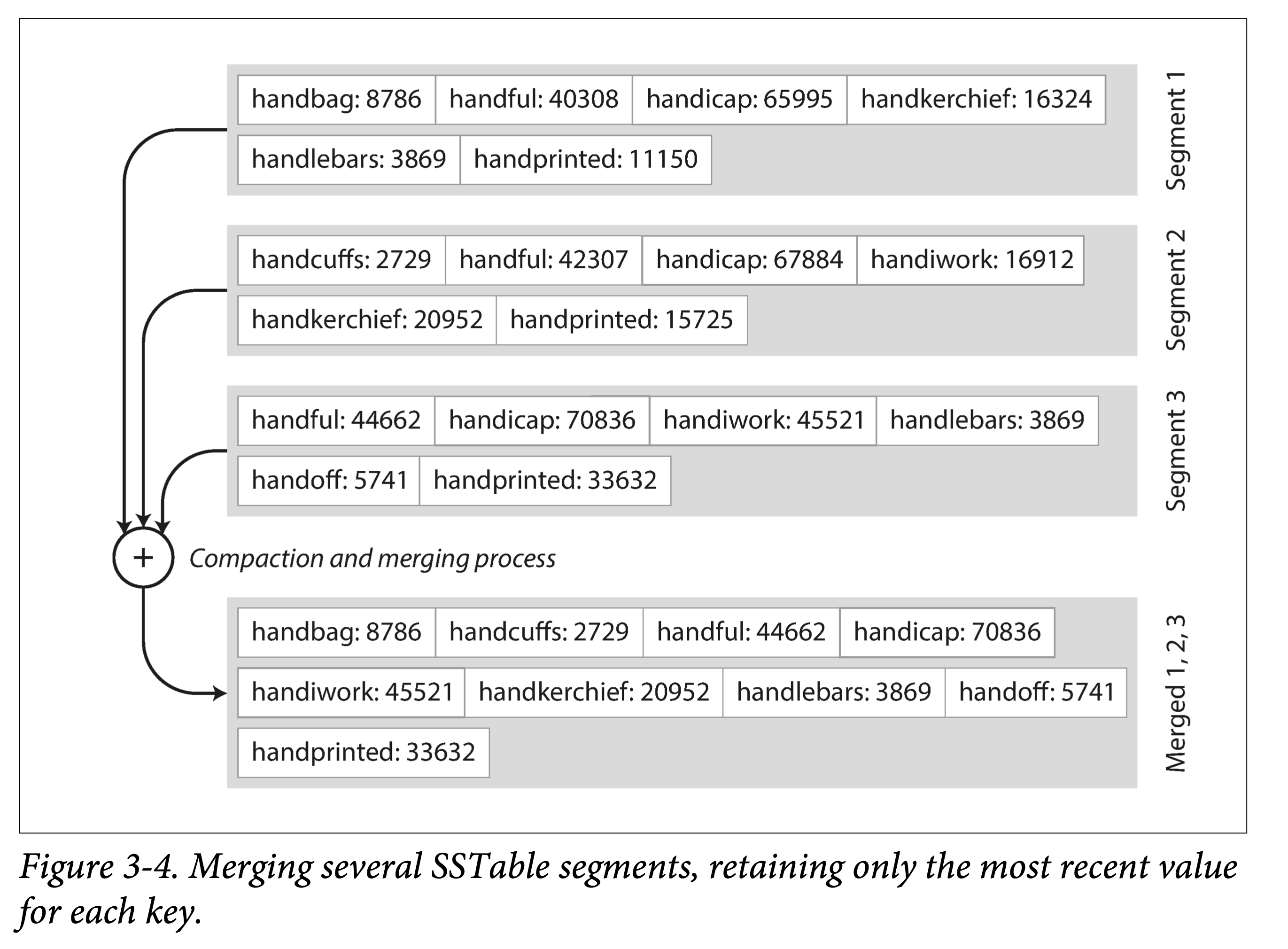ddia-3-4-merge-sst.png

No need to keep indexes for all data in memory. Only the boundaries of each file need to be recorded (represented as intervals: [startKey, endKey], though in practice finer granularity is used). When looking up a key, simply perform a binary search in the files whose intervals contain that key.

ddia-3-5-sst-index.png

Block compression saves space and reduces I/O. Adjacent keys share prefixes; since data is fetched in batches each time, a group of keys can be batched together into a block, and only the block’s index is recorded.

Building and Maintaining SSTables

The SSTables format sounds great, but we should note that data arrives out of order; how do we obtain ordered data files?

This can be broken down into two small problems:

How to build.
How to maintain.

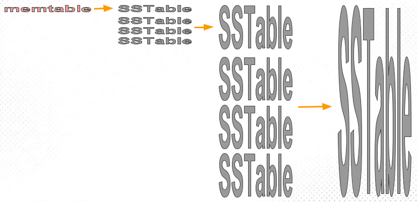
Building SSTable files. Sorting out-of-order data into ordered files on external storage (disk or SSD) is quite difficult. But it is much easier in memory. Thus a bold idea is formed:

Maintain an ordered structure in memory (called MemTable). Red-black tree, AVL tree, skip list.
Once a certain threshold is reached, fully dump it to external storage.

Maintaining SSTable files. Why is maintenance needed? First, we must ask: for the above composite structure, how do we perform queries?

First look up in the MemTable; if it hits, return.
Then search through SSTables in chronological order from newest to oldest.

If there are more and more SSTable files, the lookup cost will increase. Therefore, multiple SSTable files need to be merged to reduce the number of files, while performing GC; we call this compaction (Compaction).

Problem with this solution: if a crash occurs, the in-memory data structure will disappear. The solution is also classic: WAL.

From SSTables to LSM-Tree

Organizing the fragments from the previous sections organically gives us the storage structure behind the currently popular storage engines LevelDB and RocksDB: the LSM-Tree:

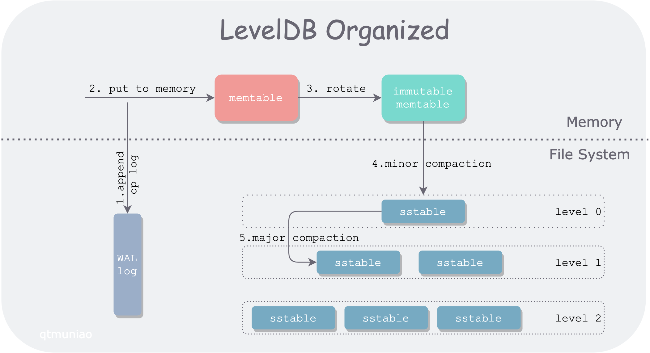ddia-3-leveldb-architecture.png

This data structure was proposed by Patrick O’Neil and others in 1996: The Log-Structured Merge-Tree.

The indexing engine Lucene used by Elasticsearch and Solr also uses a storage structure similar to LSM-Tree. But its data model is not KV, though similar: word → document list.

Performance Optimizations

If you want to make an engine usable in practice, a lot of performance optimizations are needed. For LSM-Tree, these include:

Optimizing SSTable lookups. Commonly used is the Bloom Filter. This data structure can use a small amount of memory to create some fingerprints for each SSTable, serving as a preliminary filter.

Hierarchical organization of SSTables. To control the order and timing of compaction. Common approaches are size-tiered and leveled compaction. LevelDB is named after supporting the latter. The former is relatively simple and crude, while the latter has better performance and is therefore more common.

ddia-sized-tierd-compact.png

For RocksDB, there are many more engineering and usage optimizations. Here are a few excerpts from its Wiki:

Column Family
Prefix compression and filtering
Key-value separation, BlobDB

But no matter how many variants and optimizations there are, the core idea of LSM-Tree—maintaining a set of reasonably organized, background-merged SSTables—is simple yet powerful. It allows convenient range traversal and can turn large amounts of random I/O into small amounts of sequential I/O.

B-Trees

Although LSM-Tree was discussed first, it is much newer than B+ trees.

After B-trees were proposed by R. Bayer and E. McCreight in 1970, they quickly became popular. Now in almost all relational databases, they are the standard implementation of data indexes.

Like LSM-Tree, it also supports efficient point lookups and range queries. But it uses a completely different organization.

Its characteristics are:

Organized in units of pages (called page on disk, block in memory, usually 4k).
Pages reference each other logically by page ID, thus forming a tree on disk.

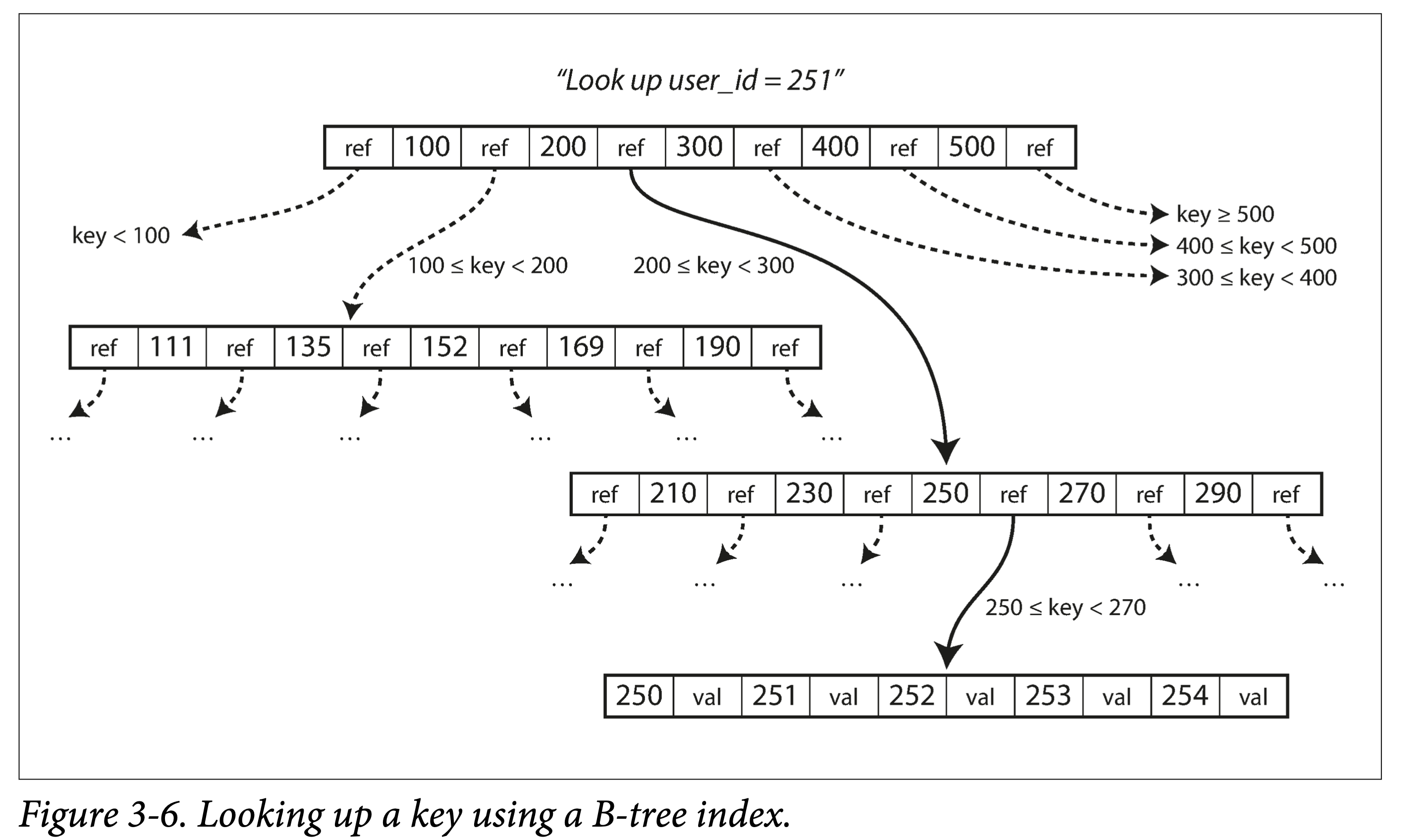ddia-3-6-b-tree-lookup.png

Lookup. Starting from the root node, perform binary search, then load a new page into memory, continue binary search, until hitting or reaching a leaf node. Lookup complexity is the height of the tree—O(log n). The factor affecting tree height: branching factor (number of branches, usually hundreds).

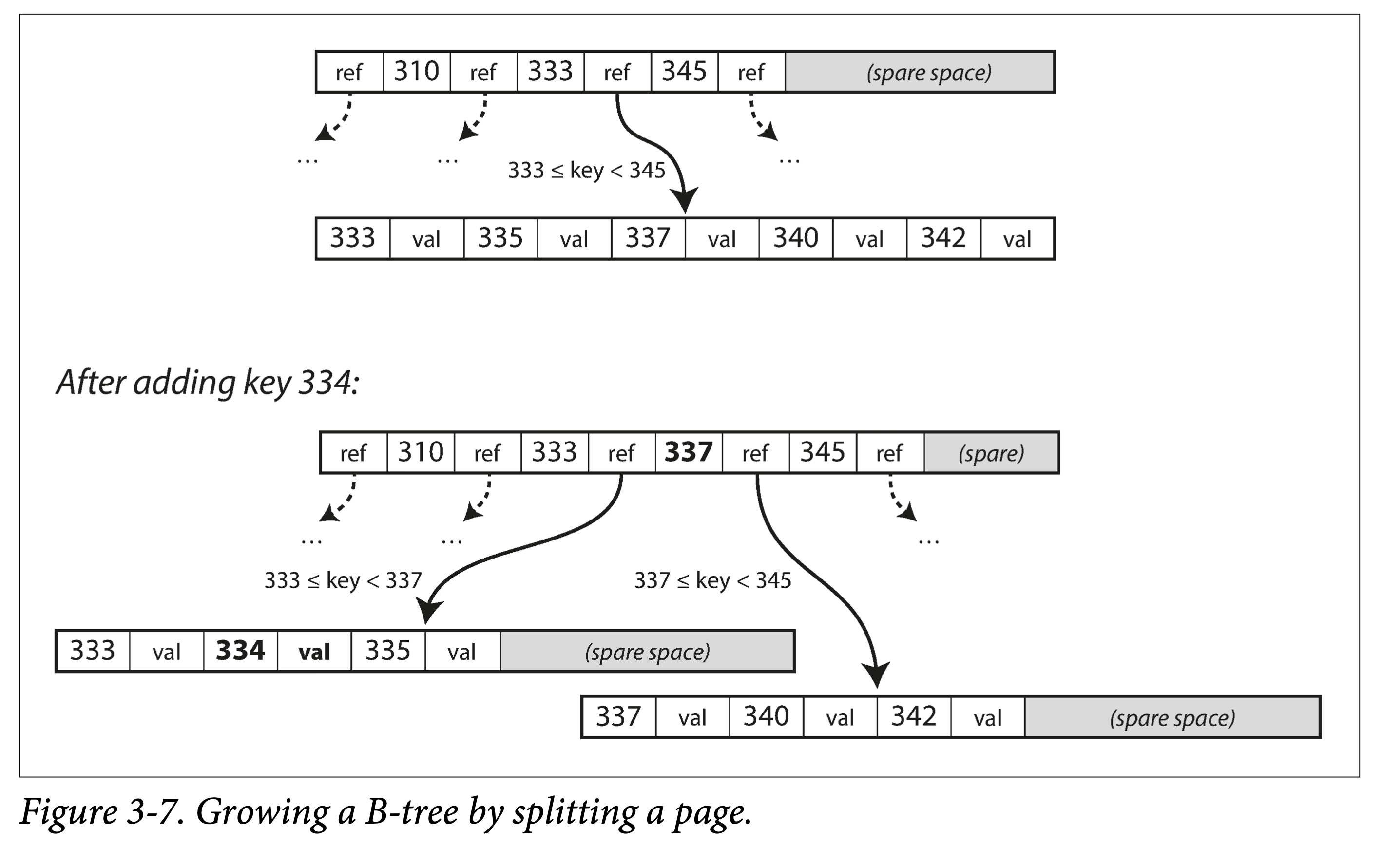ddia-3-7-b-tree-grow-by-split.png

Insert or update. Same as the lookup process: locate the page where the original key resides, insert or update, then write the entire page back. If the remaining space in the page is insufficient, split and then write.

Split or merge. Cascading splits and merges.

What if a record is larger than a page?

Tree nodes are logical concepts; page or block is a physical concept. One logical node can correspond to multiple physical pages.

Making B-Trees More Reliable

Unlike LSM-Tree, B-trees modify data files in place.

When adjusting tree structure, many pages may be modified in cascade. For example, after a leaf node splits, two new leaf nodes and a parent node (updating leaf pointers) need to be written.

Add a write-ahead log (WAL) to record all modification operations, preventing a messy state caused by interrupted tree structure adjustments during a crash.
Use latches for concurrency control on the tree structure.

B-Tree Optimizations

B-trees have been around for so long, so there are many optimizations:

Do not use WAL, but instead use Copy-on-Write technology during writes. This also facilitates concurrency control. Examples: LMDB, BoltDB.
Compress keys in intermediate nodes, keeping only sufficient routing information. This saves space and increases the branching factor.
To optimize range queries, some B-tree variants store leaf nodes physically contiguous. But as data is continuously inserted, the cost of maintaining this ordering is very high.
Add sibling pointers to leaf nodes to avoid backtracking during sequential traversal. This is the approach of B+ trees, but by no means limited to B+ trees.
A B-tree variant, the fractal tree, borrows some ideas from LSM-trees to optimize seeks.

Comparing B-Trees and LSM-Trees

Storage Engine	B-Tree	LSM-Tree	Notes
Advantage	Faster reads	Faster writes
Write amplification	1. Data and WAL 2. Multiple overwrites of the entire page when changing data	1. Data and WAL 2. Compaction	SSDs cannot be erased too much. Therefore, SSD internal firmware also mostly uses log-structured approaches to reduce random small writes.
Write throughput	Relatively low: 1. Large amount of random writes.	Relatively high: 1. Lower write amplification (depends on data and configuration) 2. Sequential writes. 3. More compact.
Compression ratio	1. More internal fragmentation.	1. More compact, no internal fragmentation. 2. Greater compression potential (shared prefixes).	But delayed compaction can cause LSM-Tree to accumulate a lot of garbage
Background traffic	1. More stable and predictable, not affected by sudden background compaction traffic.	1. If write throughput is too high and compaction can’t keep up, read amplification worsens. 2. Since total external storage bandwidth is limited, compaction affects read/write throughput. 3. As data grows, compaction’s impact on normal writes increases.	RocksDB writing too fast can cause write stall, i.e., limiting writes in order to compact data down as soon as possible.
Storage amplification	1. Some pages are not fully used	1. The same key stored multiple times
Concurrency control	1. The same key only exists in one place 2. Tree structure makes range locks easy.	The same key is stored multiple times; usually controlled using MVCC.

Other Indexing Structures

Secondary indexes. That is, the mapping from other non-primary-key attributes to the element (rows in SQL, documents in MongoDB, and vertices and edges in graph databases).

Clustered Indexes and Non-Clustered Indexes

For storing data and organizing indexes, we have multiple choices:

Data itself is stored unordered in a file, called a heap file; the value in the index points to the corresponding data’s position in the heap file. This avoids data copying when there are multiple indexes.
Data itself is stored ordered by a certain field, usually the primary key. Then the index based on this field is called a clustered index; from another perspective, the index and data are stored together. Then indexes based on other fields are non-clustered indexes, which only store references to the data in the index.
Some columns are embedded in the index for storage, while some column data is stored separately. This is called a covering index or index with included columns.

Indexes can speed up query performance, but they need to occupy extra space, sacrifice some update overhead, and need to maintain some consistency.

Multi-Column Indexes (Multi-column indexes).

In real life, combined queries on multiple fields are more common. For example, querying merchants within a certain range around a user requires a two-dimensional query on longitude and latitude.

1 2	SELECT * FROM restaurants WHERE latitude > 51.4946 AND latitude < 51.5079 AND longitude > -0.1162 AND longitude < -0.1004;

You can:

Encode two dimensions into one dimension, then store as a normal index.
Use special data structures, such as R-trees.

Full-Text Search and Fuzzy Indexes.

The indexes mentioned above only provide exact matching of full fields, not search engine-like functionality. For example, querying by words contained in a string, or querying for misspelled words.

In engineering, the Apace Lucene library and the services built around it, such as Elasticsearch, are commonly used. It also uses a log-structured storage structure similar to LSM-tree, but its index is a finite state automaton, behaving similarly to a Trie.

In-Memory Data Structures

As memory cost per unit decreases, and even with persistence support (non-volatile memory, NVM, such as Intel’s Optane), in-memory databases are gradually becoming popular.

Depending on whether persistence is needed, in-memory data can be roughly divided into two categories:

No persistence needed. Such as Memcached, which is only used for caching.
Persistence needed. Data is persisted through WAL, periodic snapshots, remote backups, etc. But all reads and writes are processed in memory, so it is still an in-memory database.

VoltDB, MemSQL, and Oracle TimesTen are in-memory databases providing relational models. RAMCloud is a KV database providing persistence guarantees. Redis and Couchbase only provide weak persistence guarantees.

The reason in-memory databases have advantages is not only because they don’t need to read from disk, but more importantly, they don’t need the extra overhead of serializing and encoding data structures to adapt to disk.

Of course, in-memory databases also have the following advantages:

Provide richer data abstractions. Such as sets and queues, which are data abstractions that only exist in memory.
Relatively simple implementation. Because all data is in memory.

In addition, in-memory databases can also provide storage space larger than physical machine memory through a mechanism similar to operating system swap. But because they have more database-related information, they can make the granularity of swapping in and out finer and performance better.

Storage engines based on non-volatile memory (non-volatile memory, NVM) have also been a hot research topic in recent years.

我是青藤木鸟，一个喜欢摄影、专注大规模数据系统的程序员，欢迎关注我的公众号：“木鸟杂记”，有更多的分布式系统、存储和数据库相关的文章，欢迎关注。关注公众号后，回复“资料”可以获取我总结一份分布式数据库学习资料。回复“优惠券”可以获取我的大规模数据系统付费专栏《系统日知录》的八折优惠券。

我们还有相关的分布式系统和数据库的群，可以添加我的微信号：qtmuniao，我拉你入群。加我时记得备注：“分布式系统群”。另外，如果你不想加群，还有一个分布式系统和数据库的论坛（点这里），欢迎来玩耍。