DDIA Reading Notes (3): TP, AP, and Column Storage

DDIA reading group. We will go through the book chapter by chapter, supplementing details based on my experience with distributed storage and databases in industry. Sharing every two weeks or so. Welcome to join us. The schedule and all transcripts are here. We have a corresponding distributed systems & database discussion group, and notifications will be sent in the group before each sharing session. If you would like to join, you can add me on WeChat: qtmuniao. Please briefly introduce yourself and mention: Distributed Systems Group.

Transactional or Analytical

The term OL (Online) mainly refers to interactive queries.

The term transaction has some historical origins. Early database users were mostly involved in commercial trades, such as buying, selling, paying salaries, and so on. But as database applications continued to expand, “transaction” remained as a noun.

Transactions don’t necessarily have ACID properties. Transactional processing is mostly random reads and writes with low latency. In contrast, analytical processing is mostly periodic batch processing with higher latency.

Author: Muniao’s Notes https://www.qtmuniao.com/2022/04/16/ddia-reading-chapter3-part2 Please indicate the source when reposting

The table below is a comparison:

Property	OLTP	OLAP
Main read pattern	Random reads of small data volumes, queried by key	Large data volume aggregation (max, min, sum, avg) queries
Main write pattern	Random access, low-latency writes	Bulk import (ETL) or streaming writes
Main application scenario	End users accessing via web	Internet analytics, to aid decision-making
How data is viewed	Latest state at the current point in time	Evolving over time
Data size	Usually GB to TB	Usually TB to PB

Initially, traditional databases were still used for AP scenarios. At the model level, SQL is flexible enough to basically meet AP query needs. But at the implementation level, the performance of traditional databases under AP workloads (low throughput for large data volumes) was unsatisfactory. Therefore, people began to turn to specially designed databases for AP queries, which we call Data Warehouses (Data Warehouse).

Data Warehouse

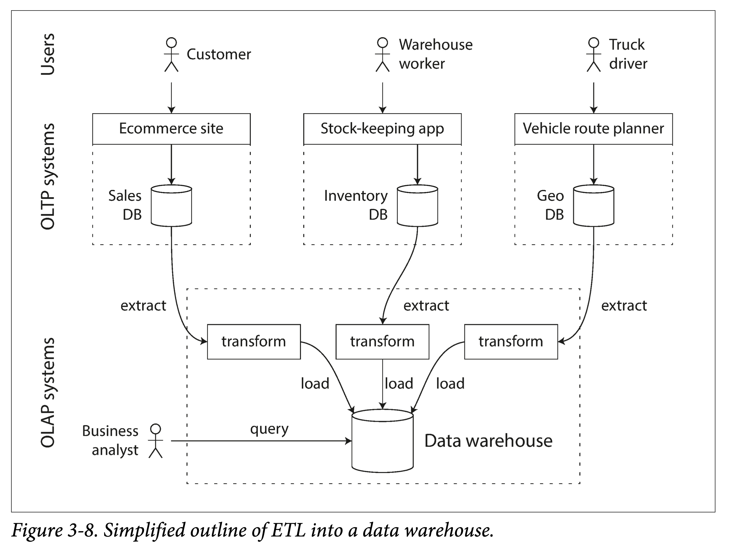
For an enterprise, there are generally many transaction-oriented systems, such as user websites, cashier systems, warehouse management, supply chain management, employee management, and so on. These usually require high availability and low latency, so performing business analysis directly on the original database would greatly impact normal workloads. Therefore, a means is needed to import data from the original database into a dedicated data warehouse.

We call this ETL: extract-transform-load.

ddia-3-8-etl.png

Generally, only when an enterprise’s data volume reaches a certain scale does it need AP analysis. After all, at a small data scale, using Excel for aggregation queries is sufficient. Of course, a current trend is that with the proliferation of mobile internet and IoT, the types and numbers of connected terminals are increasing, and the resulting data growth is also getting larger. Even relatively new startups may accumulate large amounts of data and consequently need AP support.

Aggregation queries in AP scenarios differ from traditional TP workloads. Therefore, the ways indexes need to be built also differ.

Differences Behind the Same Interface

Both TP and AP can use the SQL model for querying and analysis. However, because their workload types are completely different, the design decisions made when implementing query engines and optimizing storage formats also differ greatly. Therefore, beneath the surface of the same SQL interface, the underlying database implementation structures of the two are quite different.

Although some database systems claim to support both, such as earlier Microsoft SQL Server and SAP HANA, they are also increasingly evolving into two independent query engines. HTAP systems, which have been mentioned more frequently in recent years, are similar. To serve different types of workloads, they actually have two different storage engines at the bottom layer. It is just that the system internally automatically handles data redundancy and reorganization, transparent to the user.

AP Modeling: Star and Snowflake Schemas

There are relatively few processing models in AP. A commonly used one is the star schema, also known as the dimensional model.

ddia3-9-star-schema.png

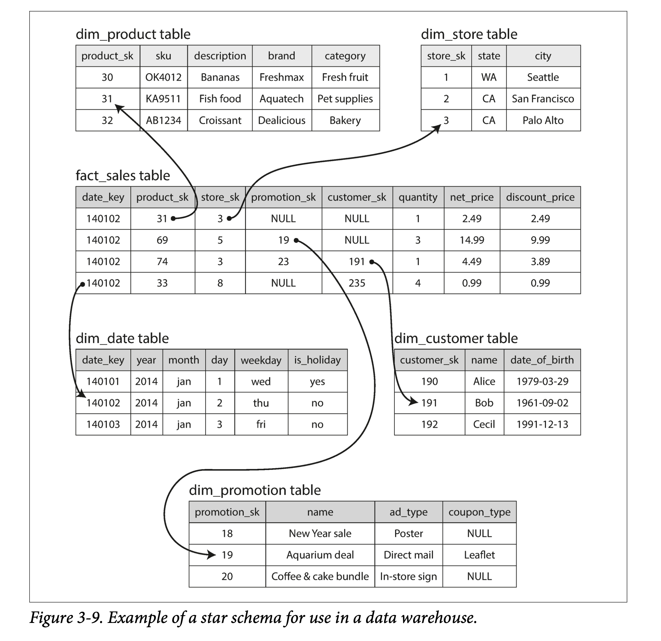
As shown in the figure above, the star schema usually contains one fact table and multiple dimension tables. The fact table organizes data in the form of an event stream, and then points to different dimensions through foreign keys.

A variant of the star schema is the snowflake schema, which can be analogized to a snowflake (❄️) pattern. Its characteristic is that dimension tables are further subdivided, breaking a dimension into several sub-dimensions. For example, brand and product category may have separate tables. The star schema is simpler, while the snowflake schema is more refined; different trade-offs are made in specific applications.

In a typical data warehouse, the fact table may be very wide, that is, having many columns: from one hundred to several hundred.

Column Storage

The dimension tables and fact tables mentioned in the previous section—for the latter, they may reach billions of rows and several PB in size. Although fact tables may typically have dozens or hundreds of columns, a single query usually only focuses on a few dimensions (columns).

For example, querying whether people are more inclined to buy fresh fruit or candy on a particular day of the week:

SELECT
  dim_date.weekday,
  dim_product.category,
  SUM(fact_sales.quantity) AS quantity_sold
FROM fact_sales
  JOIN dim_date ON fact_sales.date_key = dim_date.date_key
  JOIN dim_product ON fact_sales.product_sk = dim_product.product_sk
WHERE
  dim_date.year = 2013 AND
  dim_product.category IN ('Fresh fruit', 'Candy')
GROUP BY
  dim_date.weekday, dim_product.category;

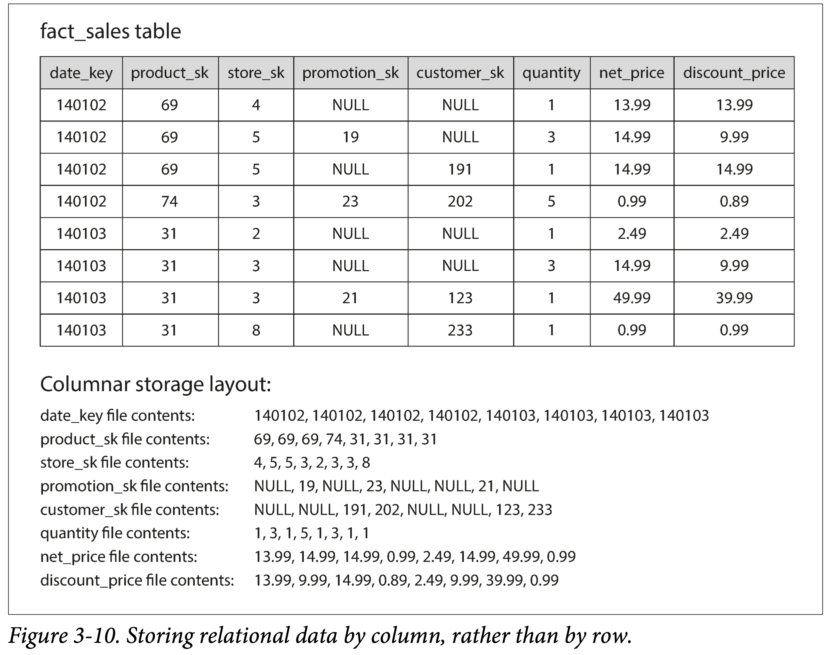
Since traditional databases usually store data by row, this means that for tables with many attributes (columns), even if only one attribute is queried, many attributes must be fetched from disk, undoubtedly wasting IO bandwidth and increasing read amplification.

Thus, a very natural idea emerges: how about storing each column separately?

ddia-3-10-store-by-column.png

Fields in the same row across different columns can be matched by index. Of course, an embedded primary key could also be used for matching, but that would make storage costs too high.

Column Compression

Storing all data in separate columns brings an unexpected benefit: because data of the same attribute has high similarity, it is easier to compress.

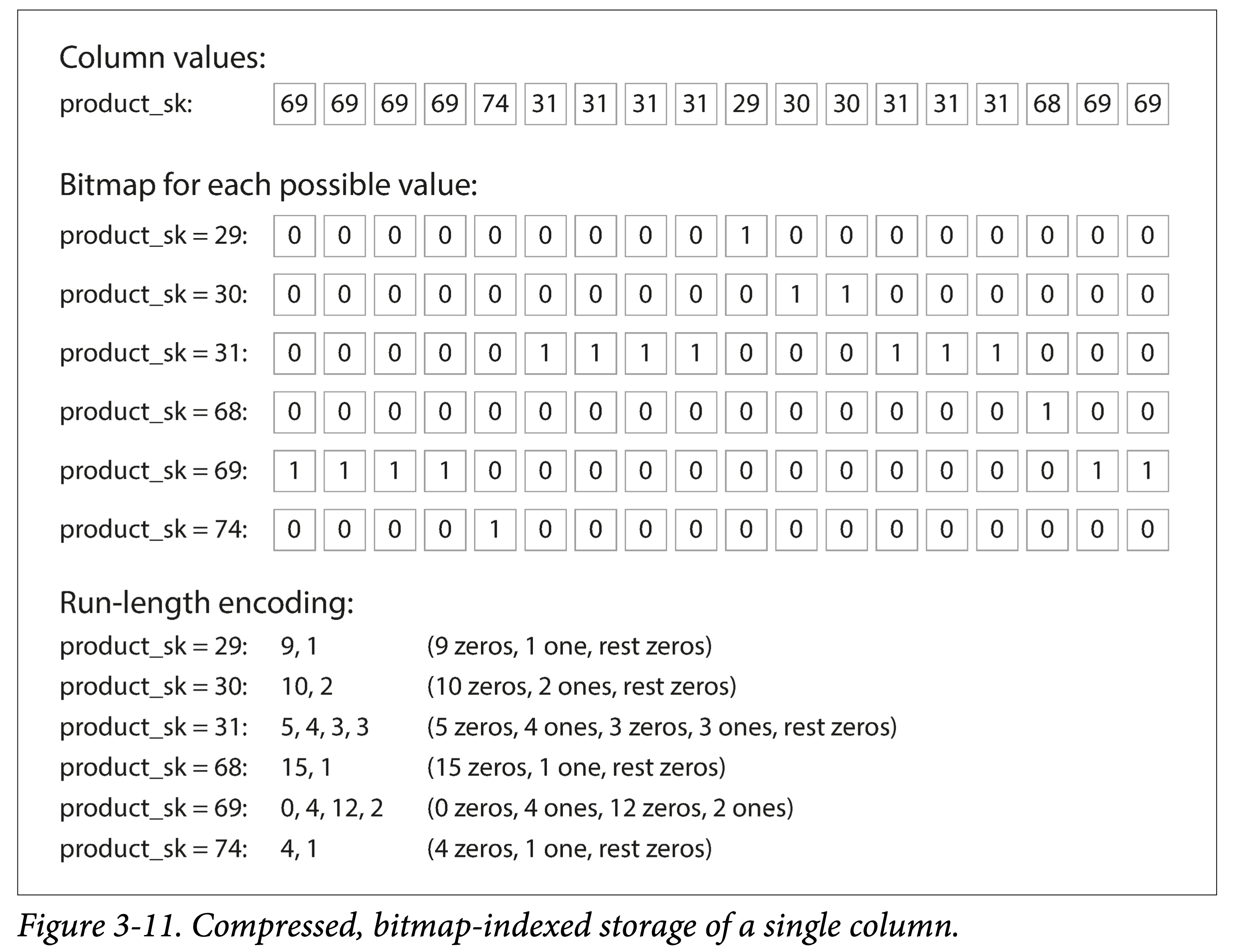
If the number of distinct values in each column is much smaller than the number of rows, bitmap encoding can be used. For example, a retailer may have billions of sales transactions, but only 100,000 distinct products.

ddia-3-11-compress.png

In the figure above, the data in a column fragment shows only six distinct values: {29, 30, 31, 68, 69, 74}. For each value’s occurrence positions, we use a bit array to represent them:

1. The bit map index corresponds to the column index.
2. A value of 0 means the value does not appear at that index.
3. A value of 1 means the value appears at that index.

If the bit array is sparse, that is, mostly 0s with only a few 1s, Run-length encoding (RLE, Run-length encoding) can also be used for further compression:

1. Rewrite consecutive 0s and 1s as count+value. For example, product_sk = 29 is 9 zeros, 1 one, 8 zeros.
2. Using a small trick to further compress the information. For example, after merging same values, they must appear in an alternating pattern of 0 and 1. If the first value is fixed as 0, then the alternating 0s and 1s don’t need to be written either. Thus, product_sk = 29 is encoded as 9, 1, 8.
3. Since we know the bit array length, the last number can also be omitted, because it can be obtained by array len - sum(other lengths). Thus, the final encoding for product_sk = 29 becomes: 9, 1.

Bitmap indexes are well suited for logical operation conditions in queries, such as:

WHERE product_sk IN (30, 68, 69)

Can be converted to a bitwise OR of the three bit arrays for product_sk = 30, product_sk = 68, and product_sk = 69.

WHERE product_sk = 31 AND store_sk = 3

Can be converted to a bitwise AND of the bit arrays for product_sk = 31 and store_sk = 3, to get all the required positions.

Column Families

The book specifically mentions column families. It is a concept in Cassandra and HBase, both of which originated from Google’s BigTable. Note that they have similarities with column-oriented storage, but are definitely not the same:

1. Multiple columns in the same column family are stored together, with the row key embedded.
2. And columns are not compressed (questionable?)

Therefore, BigTable is still mainly row-oriented when in use. It can be understood that each column family is a sub-table.

Memory Bandwidth and Vectorized Processing

The ultra-large scale data volume of data warehouses brings the following bottlenecks:

1. Memory processing bandwidth
2. CPU branch prediction misses and pipeline stalls

Memory bottlenecks can be alleviated through the data compression mentioned earlier. For CPU bottlenecks, we can use:

1. Columnar storage and compression allow as much data as possible to be cached in L1, combined with bitmap storage for fast processing.
2. Use SIMD to process more data with fewer clock cycles.

Sorting in Columnar Storage

Since data warehouse queries mostly focus on aggregation operators (such as sum, avg, min, max), the storage order in columnar storage is relatively unimportant. But it is also unavoidable to filter certain columns using conditions. For this, we can, like LSM-Tree, sort all rows by a certain column and then store them.

Note, it is impossible to sort on multiple columns simultaneously. Because we need to maintain the index correspondence between multiple columns in order to fetch data by row.

At the same time, the sorted column will have better compression effects.

Different Replicas, Different Sort Orders

In distributed databases (data warehouses are so large that they are usually distributed), we store multiple copies of the same data. For each copy, we can store it sorted by different columns. Thus, for different query needs, we can route to different replicas for processing. Of course, this way we can at most build column indexes equal to the number of replicas (usually around 3).

This idea was introduced by C-Store and adopted by the commercial data warehouse Vertica.

Writes to Columnar Storage

The above optimizations for data warehouses (columnar storage, data compression, and sorting by column) are all aimed at solving the common read-write workloads in data warehouses: read-heavy, write-light, and reads are all ultra-large scale data.

We optimized for reads, which makes writes relatively difficult.

For example, B-tree’s in-place update flow doesn’t work well. For instance, to insert data in the middle of a row, vertically speaking, it would affect all column files (if not segmented); to ensure index correspondence between multiple columns, horizontally speaking, all column files for the different columns of that row would also need to be updated.

Fortunately, we have LSM-Tree’s append-only flow.

1. Batch newly written data in memory, by row or by column—what data structure to choose depends on requirements.
2. Then, after reaching a certain threshold, flush it in batches to external storage and merge it with old data.

The data warehouse Vertica does exactly this.

Aggregation: Data Cubes and Materialized Views

Not all data warehouses are columnar stores, but the many benefits of columnar storage have made it popular.

One of them worth mentioning is materialized aggregates (or materialized summaries).

Materialized can be simply understood as persisted. Essentially, it is a space-for-time tradeoff.

Data warehouse queries usually involve aggregation functions, such as COUNT, SUM, AVG, MIN, or MAX in SQL. If these functions are used multiple times, computing them on the fly every time is obviously a huge waste. Therefore, an idea is: can we cache them?

The difference from views in relational databases is that views are virtual, logical existences, just an abstraction provided to users, an intermediate result of a query, and are not persisted (whether there is caching is another matter).

Materialized views are essentially a summary storage of data. If the original data changes, the view needs to be regenerated. Therefore, if writes are heavy and reads are light, the cost of maintaining materialized views is high. But in data warehouses it is often the opposite, which is why materialized views can work well.

A specialized example of materialized views is the data cube (or OLAP cube): aggregating quantitative data by different dimensions.

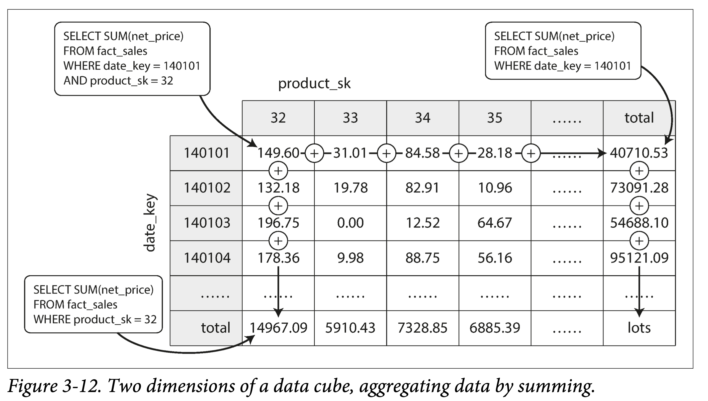ddia-3-12-data-cube.png

The figure above is a data cube summed by two dimensions: date and product category. When performing summary queries by date and product, due to the existence of this table, it becomes very fast.

Of course, in reality, a table often has multiple dimensions. For example, in Figure 3-9 there are five dimensions: date, product, store, promotion, and customer. But the meaning and method of building data cubes are similar.

But such constructed views can only optimize for fixed queries. If some queries are not among them, these optimizations no longer work.

In practice, it is necessary to specifically identify (or estimate) the query distribution for each scenario, and build materialized views accordingly.

---

我是青藤木鸟，一个喜欢摄影、专注大规模数据系统的程序员，欢迎关注我的公众号：“木鸟杂记”，有更多的分布式系统、存储和数据库相关的文章，欢迎关注。 关注公众号后，回复“资料”可以获取我总结一份分布式数据库学习资料。 回复“优惠券”可以获取我的大规模数据系统付费专栏《系统日知录》的八折优惠券。

我们还有相关的分布式系统和数据库的群，可以添加我的微信号：qtmuniao，我拉你入群。加我时记得备注：“分布式系统群”。 另外，如果你不想加群，还有一个分布式系统和数据库的论坛（点这里），欢迎来玩耍。